License
This work is licensed under the Creative Commons Attribution-ShareAlike 4.0 International (CC BY-SA 4.0) License. To view a copy of this license, visit https://creativecommons.org/licenses/by-sa/4.0/ or send a letter to Creative Commons, PO Box 1866, Mountain View, CA 94042, USA.
Copyright 1995 Paul Overaa
The Author
Paul Overaa initially qualified as an analytical chemist and spent two decades working in a field of physical chemistry known as gas-liquid chromatography. It was during this time that he became heavily involved with computerised data reduction techniques and computer programming. Nowadays he considers himself a programmer first and an analytical chemist second.
Paul has previously written books on low-level 6502 and Z80 assembly language programming, on Amiga programming in C and ARexx, and on both Amiga and Atari ST program design. He is a proficient C and 68000 assembly language coder, and an experienced Amiga programmer. As a technical author he also writes for a great many computer programming magazines and periodicals including Amiga Shopper, Amiga User International, Amiga Computing, and Computing. In the past he has worked for Amiga Format, Program Now, ST World, Atari ST User and the one time highly influential Transactor Amiga magazine.
In addition to computing columns he also provides expertise on MIDI programming for a variety of magazines and in the past he has written for Sound on Sound, International Musician, and many other publications. His main passion nowadays is computer programming with his research interests having a strong bias towards language-independent program design techniques. Other interests include badminton, yoga, mathematics and, when he has time and the weather on his side, windsurfing.
Introduction
You’ve either bought this book already or are giving it the once over to see whether it will be useful to you or not. If you’ve already bought it then thanks, I’m sure you will not be disappointed. If, on the other hand you are still deciding, then the following notes outlining the overall plan of the book should help you to make up your mind.
To start let me point out that learning an assembly language is not in itself a difficult task. I’ll be the first to admit that there are many books available which have excellent introductory accounts of this subject. But a microprocessor does not work in isolation and in the Amiga the 680x0 processor is just a small part of a complex system which involves not only a great many other hardware components but a very complex covering shell of operating system software as well. If you are intent on programming the Amiga using 680x0 assembly language then some knowledge of this operating system is needed right from the start and this produces an immediate stumbling block.
Almost all books which deal in depth with programming the 680x0 microprocessors do so in an operating system independent way and this makes it very difficult for the would-be Amiga assembly language programmer to relate what they are learning about to the Amiga environment. On the face of it the solution would be to use general 680x0 books to learn about programming the processor and get the Amiga-specific material from books which deal specifically with the Amiga’s operating system. Things are not however quite that simple because much of the Amiga’s documentation has been written with the C programmer in mind. Worse than that, much of it has been written for professional programmers who are already system literate.
The bottom line is that in many ways newcomers to assembly language, no matter how enthusiastic they might be, are left high and dry and it is exactly this information gap which I have tried to fill with this book. I’ve attempted to introduce 680x0 assembly language specifically from an Amiga orientated viewpoint and my main aim has been to provide you with the necessary footholds to get into low-level Amiga programming as quickly as possible. Having said that this is not purely a beginners book - I’ve included details about a number of areas of more advanced nature. The reason is simply that I wanted this book to remain useful to you a long time after you’ve taken your first steps into the world of assembly language coding.
The material in this book is essentially self-contained but as you progress you will doubtless follow your own path in terms of what you choose, Amiga-wise, to take an interest in. Regardless of the directions in which you travel you will almost certainly get to a point where more and more reliance has to be placed on the Amiga’s official system documentation. I would be less than honest if I told you that some experience with the C language would not be an advantage to you at this stage and my experience is that all programmers, including those whose sole interest was programming at the 680x0 microprocessor level, have eventually needed to come to terms with C just in order to cope with the official Amiga documentation. This, from a long term viewpoint, is something which you should clearly keep in mind.
I will not be using, or referring to the C language, for the bulk of this book but there a few occasions, such as the example on mixed code programming, where some knowledge of C is needed. Because of this, and because you may find the material generally useful in your Amiga travels, I have included a small appendix which outlines the most important features of the C language.
As far as learning 680x0 assembler goes I have worked primarily on a need to know basis and have concentrated on those Amiga specific topics that are not found in more general 680x0 books and which, in my opinion, have not been properly explained (from the beginner’s viewpoint) in existing Amiga specific texts. In order to gain sufficient space to do this I’ve avoided duplicating what I regard as essentially standard 680x0 information. You will not, for instance, find detailed accounts of each and every instruction that the 680x0 range of processors can execute (such material is readily available from the sources mentioned in the bibliography).
Similarly I have avoided extended discussions of hardware issues because to start assembler programming on the Amiga, and any other machine come to that, all that is needed is a simple conceptual model of the processor and its facilities. Knowledge of how the processor physically communicates with memory and the outside world, and discussions of what timing signals are used to ensure that such things happen at the right time, are two example areas which do not seem to facilitate the move to low-level programming. These hardware related topics are certainly important to system designers and engineers but for most would-be assembler programmers I’ve found that discussions of such material only complicates matters.
In short then I’ve attempted to isolate you the reader from any low-level topic that does not directly contribute to the real task at hand, namely how to go about writing your first 680x0 programs.
For many years, right up to and including Workbench 1.3, the Amiga’s operating system was relatively stable in terms of it’s core library functions. Sure there were various additions made but none of this really affected anything that a new low-level Amiga coder needed to worry about. In recent years, most notably with Release 2 of the operating system, things changed fairly dramatically and a number of changes are so fundamental that they cannot be skipped over, even by the newcomer. The introduction of things called Tag Lists for example has changed the way that the setting up of Amiga screens and windows are coded from assembler. Similarly the arrival of a system library called GadTools has had a big influence on the ‘flavour’ of much Amiga code. All these things are now an integral part of modern Amiga coding and whether you’re writing code for Release 2 or the new Workbench 3 arrangements, it’s important to understand them. Needless to say you’ll find all these things and more explained in this latest book.
So, there is plenty of material suitable for the beginner but in addition to this I’ve also included various topics of more advanced nature. You’ll find details of how to create code that is ‘pure’ (ie can be made resident), how to create Exec style run-time libraries. I’ve even included details of how to build an assembly language coded function library that can be called from ARexx!
All in all then there should be something for everyone but of course the initial task is to provide the footholds for the beginner wishing to learn about Amiga 680x0 assembly language programming. If, incidentally, you are new to this subject then please take heart – I believe that I can not only show you a simple pathway to achieve this objective but that I’ll even be able to make the subject enjoyable and that, believe me, is over half of the battle!
Paul Overaa, 1995
In the listings printed in this book you will find curly “ and ” characters. These represent the ” (straight) quote marks which you get when pressing the Amiga key <Shift-2>.
1. Fundamental Concepts
The objective of this chapter is to draw your attention to, and explain, a number of general issues related to the writing of assembly language programs. As you probably know, the heart of the conventional microcomputer system is a combined logic/control unit known as a central processing unit or CPU. Most processors have a considerable number of common characteristics including the fact that all have a set of internal registers for storing data and all have some hardware-orientated means of communicating with the outside world. Since the amount of internal storage available on the CPU itself is always limited it must, before it can do any useful work, also be connected to additional memory components that are able to provide a suitable amount of additional CPU-accessible electronic storage. Two basic types of memory chips are in common use:
RAM (random access memory) chips may be both written to and read from and as such are used to provide storage space that may be dynamically changed either prior to or during program execution.
ROM (read only memory) chips can only be read from and are therefore used to hold information blocks that do not change. Once programmed, a ROM chip, whether powered up or not, will keep its contents indefinitely. RAM chips on the other hand do not hold their data in this way and when the power is removed from the system the contents of all random access memory units will disappear.
On small and medium power computers the processor is usually an integrated circuit known as a microprocessor and this device will have its own instruction set, a collection of logic/arithmetic instructions, which can cause the microprocessor to perform various tasks. At the end of the day it is sets of these instructions, stored in memory, which constitute the programs which will be executed by the computer system.
The language that the microprocessor understands is based on binary numbers. Given suitable hardware ie, a processor chip, memory, some input/output facilities, and all the associated electronic support, one way of programming such a system would be to enter suitable binary numbers directly into system memory and then to get the microprocessor to execute the instructions.
This machine code programming approach was actually used to create and run programs in the early days of computing. It didn’t take long before programmers realised that this sort of programming was a pain because the numbers which related to particular processor instructions didn’t have any obvious connection with what the programmer was really trying to do. The solution was to give the instructions meaningful names (or as meaningful as possible) eg ADD, MOVE, SUB and so on. These humanised instruction names were called mnemonics because they were a memory aid that helped programmers to remember the purpose of the underlying processor instructions. The next step was to automate the process of converting mnemonics back to the numbers which represented the processor instructions. Programs which did this translation effectively assembled the runable program from the mnemonic instructions that the programmer had provided so they were called assemblers. In short, assembly language programming was born!
Over the years microprocessors, assembly language programming concepts, and development software have all become increasingly sophisticated but these assembly languages (and each microprocessor has its own) are always close to the actual machine and its underlying hardware – hence they are called low-level languages. The Amiga, as you’ll doubtless already know, uses microprocessors from a family of chips called the Motorola 680x0 series. The original chip from this series is the 68000 and this is what was used to build the first Amigas. Later machines, and add on accelerator cards, have used the faster and more powerful 68020, 68030 and 68040 chips but because these processors are code compatible with the original 68000 the bulk of most Amiga code written today is still written just in terms of the 68000 instruction set — simply in order that it may safely run on all Amigas.
This means of course that to conveniently program all Amigas at the microprocessor level you need to concentrate initially on learning about 68000 assembly language. It should come as no surprise therefore to hear that it is the instruction set of this chip that forms the basis of this book.
High-Level Alternative
The birth of assembly language didn’t solve all of the problems that the early programmers faced. To start with, programs written in low-level languages are processor specific so they are not portable, ie not easily made to run on different processors. Another problem is that you have to express what you want to do in terms of the instructions which are available on the processor and this means working primarily with bits and bytes. Any other data structures needed have to be created by the programmer so if, for instance, the problem being solved involved text strings or floating point numbers then it is you, the programmer, who would have to decide how to represent those entities, and do the necessary programming.
High-level languages, such as BASIC and Pascal, attempt to provide a vehicle for expressing algorithms which is more human orientated and powerful. A single statement in a high-level language might correspond to operations which, when expressed in a lower-level language, would need many hundreds of code instructions. At the end of the day however the high-level language interpreter or compiler must produce such a series of low-level machine instructions in order that the program can run.
In reality, this low-level/high-level two tier classification is rather an oversimplification. Nowadays there exists a wide spectrum of languages each possessing features from both groups. Almost all current assemblers for example allow macros, reusable groups of low-level operations, to be built up and the creation of these types of units allow the programmer to tackle low-level code writing at a significantly higher level than was possible with early assemblers. Having said that, high-level languages clearly have a number of important benefits:
-
The structure of the program can be based on, or reflect, the inherent structure of the original problem.
-
High-level languages can usually offer a degree of self-documentation.
-
High-level languages allow meaningful, hardware independent, names to be used both for data and procedures/subroutines.
-
The abstraction offered by high-level languages allows for a clearer algorithm representation. Much of the detail which would be present in a lower-level form is hidden by the more powerful language statements.
-
High-level languages are easier to learn than low-level languages.
-
High-level languages often offer sophisticated debugging facilities.
-
High-level programs are often more portable, ie can run on any machine for which the language has been implemented.
The key advantage offered by high-level languages is that they provide a means of expressing the steps of an algorithm at a more problem/solution orientated level. If, for example, you wish to open a file, read some data, and then close a file it might be possible to use program statements which represent these file opening, data reading, and file closing operations directly. Three statements which relate closely to the things which need to be done, as opposed to hundreds of assembler instructions which, taken in isolation, will give few obvious clues as to the work being carried out.
As the level of abstraction increases, the programmer becomes less concerned with the hardware on which the program runs and is able to work more and more at a problem-orientated level. Symbolic names take the place of memory addresses, support for different data types means that the language (as opposed to the programmer) can be left to figure out the details about the sizes of objects being used and how/where they should be stored. Similar generalised control abstraction facilities allow loops and decision tests to be used as building blocks, which again makes it easier for the programmer to tackle problems in a solution orientated, rather than a hardware orientated, way.
Now if these high-level language characteristics are so good why on earth are people still using assembly language at all? To be honest people have been predicting the demise of the assembly language programmer for years but it simply hasn’t happened — in fact interest in assembly language programming actually seems to be on the increase and it turns out that there is far more to the high-level/low-level debate than first meets the eye.
Low-Level Approach
It was once thought that there were only three reasons for using assembly type languages: speed, compactness and the ability to achieve the ultimate control over the system. The benefits are rather more subtle than this because there’s no doubt that an understanding of an assembly language gives the programmer an in-depth appreciation of what high-level languages must do to achieve their abstraction magic. It’s a similar situation to driving a car. If you don’t know roughly how the gears work then you might wonder why you can’t pull away in fourth gear without stalling the engine. Plenty of driving will convince you that this is indeed the case, but no matter how much you drive you’ll never actually find out why this is so. Learn a bit about the internal mechanics however and it will become obvious within a very short space of time!
Since the Amiga is a 680x0 based machine it’s not hard to figure out that all Amiga languages must end up generating 680x0 code – they have to because otherwise the final programs simply wouldn’t be able to run on the Amiga’s microprocessor. What then is it that actually makes code written by assembler programmers run faster than the equivalent 680x0 code generated by programmers working with high-level languages? The answer is simply that the assembler programmer can make sure that their final code is super-efficient. Here’s a typical example.
As you may know, the Amiga has a vast number of pre-written routines available which are organised as a collection of units known as run-time libraries. The routines present in these libraries are accessed by a table stored in memory immediately below the base (main reference) address of the library. By using a negative offset, called an LVO (Library Vector Offset), the programmer can specify which routine is to be called. These routines are used by placing the library’s base address in one of the 680x0 registers (actually register a6), using the LVO as a displacement value, and performing something called an indirect subroutine call. These terms may not mean much at the moment but the important point to grasp is that the necessary data needs to be held in the microprocessor’s internal registers before the subroutine call is made.
Now let’s consider what happens with a conventional C compiler when a high-level function call is used to execute the same library routine. The compiler starts by pushing function call parameters onto the stack, an area in memory which the microprocessor uses to store items on a last-in-first-out basis. Now, when you are calling an Amiga library function, it turns out that this is a total waste of effort because, at the end of the day and as indicated above, the Amiga run-time libraries expect the parameters to be present in the 680x0 processor registers and not on the microprocessor stack. The bottom line is that before the real library function call can occur, the parameters, so carefully placed on the stack by the compiler generated code, have to be immediately copied back into suitable processor registers.
The code stubs which do this are part of the amiga.lib library and this, plus the fact that the LVO values are also needed, is the reason why C programmers usually link their code with the amiga.lib linker library in the first place. The resultant C code therefore ends up doing a lot of unnecessary work and this of course slows the program down. By placing library call parameters directly into the appropriate 680x0 registers the assembly language programmer can eliminate such inefficiencies very easily indeed.
Now to be completely fair, at least as far as the above example goes, I ought to point out that some compilers (eg SAS C) do now support register based parameter passing and can therefore also now eliminate these amiga.lib subroutine time penalties. Being equally fair as far as the assembler programmer is concerned I should mention that while register based parameter passing in C is a recently added facility such advantages have always been available to the 680x0 assembler programmer!
The underlying general point I’m trying to make is this: all high-level languages have to make compromises with the code they generate and because of this there will always be many occasions where the assembly language programmer can cut corners and eliminate inefficiencies. This is the reason why the assembly language programmer will almost always be able to produce program code that runs faster than code generated by a compiler.
Assembly language then has a lot going for it. High-level language topics that programmers often find difficult to understand, such as bit-manipulation operations and the use of indirection and pointers, have natural and easy to recognise counterparts in assembly language. The overall result, believe it or not, is that knowing something about your machine at this low level of programming will not only help you get a gut feeling for what computing is all about but it can even help you to write more effective high-level code. For more information see the Appendix on other books in the Bruce Smith Books range.
Creating an Assembly Language Program
The first step in writing an assembly language program is to use an editor program to prepare a source code file. This file will simply be an ASCII text file which contains the program instructions that you’ve written and you will of course be able to list and print the contents of such a file just as you would a letter or any other piece of stored text. Most commercial assemblers come with their own editor programs but, if you prefer, it is also possible to use an alternative editor or wordprocessor program. The only provison with the latter option is that it must be possible to stop the wordprocessor from inserting additional control characters because these characters would, as likely as not, cause the assembler program to come to a grinding halt as it tries unsuccessfully to interpret them.
Once a source file is available, the next step is to get the assembler program to convert it to the appropriate 680x0 instructions. On the Amiga the assembler will in many cases first have to be used to create a standardised intermediate form known as an object code file. This is not a runnable program as such and there are three possible reasons for this. Firstly, although the object file will include the translated 680x0 instruction-related material, the code will not itself be in the right format to be loaded by AmigaDOS. Secondly, the program will not contain an all-important piece of Amiga specific front-end code known as the startup code which is needed if the program is to run from the Workbench. Thirdly, the file may still contain references to unresolved (unknown) items, such as linker library routines or variables that have been specified as being present in other object code modules.
A third stage, known as linking, attempts to fill in the gaps created by these unresolved references. The Amiga linker, called Blink, is able to combine the startup code and the code you have written (plus any other specified object code modules or library code), to produce a program file that may then be loaded and run under the Amiga’s operating system. Having said all that I’m afraid that I must now point out that nowadays many assemblers can produce a variety of different output file formats. HiSoft’s Devpac assembler for instance, providing it is presented with a suitable source code file, can generate directly executable code without an explicit linking stage!
Libraries on the Amiga cause a few headaches for the beginner primarily because the term is used in a number of different ways. During the example of high-level language inefficiencies I spoke of the Amiga’s runtime libraries which are collections of shared routines that, by virtue of the Amiga’s operating system, can be made available to all programs which need them during the times that they are actually running.
The libraries I am talking about in the context of the above linker discussion are rather different. Linker libraries are sets of pre-written system or utility routines which will be tagged onto the code you write during the linking stage. If you use a linker library function within your program the linker, providing you correctly specify the name of the library which holds the routine, will automatically find and include the right piece of code in the finished program. I’ll be saying much more about the various Amiga library schemes later in the book.
On occasion things may not go well and you may find that as the assembler attempts to translate your source file it reports any number of errors. Whatever the cause (syntax errors, illegal instructions etc) these faults will have to be corrected and this may mean that in the early days you’ll frequently pass through the edit<->assemble cycle quite a few times before you succeed in creating a program that assembles successfully. Even having got through that stage of the proceedings you may then find that the linker reports additional errors. Mis-spelling library routine names or not specifying the correct location of library files are commonly seen linker errors. These errors must also be found and eliminated before a runable version of the program can be created.
As you doubtless already know there is no guarantee, even once a program is up and running, that it is free from errors. In fact assembly language programmers, unless they are very careful, are likely to spend far more time looking for bugs than their high-level language counterparts. Many assembly language programmers frequently use a piece of software called a debugger, which is a system tool that is able to execute a program on a step-by-step basis, in order to help them to trace program execution and identify faults. Whilst I certainly agree that debuggers can be useful on occasion I am not in favour of their use as a general fault-finding tool.
Number Systems
One thing you are going to need to get used to as you enter the world of assembly language is the use of additional numbering systems. Since this primarily involves binary and hexadecimal numbers some words on these two number schemes are in order.
In the decimal number system ten different symbols (the digits 0-9 inclusive) are used to represent numbers. Each digit in a number is ten times more significant than the digit to its right, and ten times less significant than the digit to its left. This ten times relationship that exists between the digits of all decimal numbers is obviously a fundamental part of the decimal numbering system. If, for example, we consider the number 375 and write a full description of what each digit means, we can see that it is just a convenient way of expressing this sum:
(3x100) + (7x10) + 5
Going one better than this and, bearing in mind that any number raised to the power zero is unity, you can express each effective digit term as a product of one digit and a power of 10 like this:
3x10² + 7 x 101 + 5x100
For decimal numbers 10 is known as the radix, or base, of the numbering system but many other bases are possible. Computers use binary, ie base 2, numbers which consist of strings of Os and 1s and again, if you think of a binary number in terms of its explicit radix = 2 representation, it’s easy to see the relationship between the binary and decimal number systems:
1 |
0 |
1 |
1 |
binary = |
1x23 |
0x22 |
1x21 |
1x20 |
|
8 |
0 |
2 |
1 |
= 11 decimal |
By writing out what the binary number means in full it becomes quite easy to see that 1011 binary is the decimal number eleven!
Computers use binary numbers internally because the two digits 0 and 1 relate directly to the possible states of bits within the memory hardware of most computer systems. Binary numbers are then intimately involved with a great many computing applications but, since they are not that easy for us humans to work with (because long strings of Os and 1s are easily mis-interpreted) a related radix scheme called hexadecimal is often used as an alternative. Hexadecimal numbers use a radix of 16 and the sixteen symbols used are the digits 0-9 plus the letters A-F. Each column in a base 16 number therefore represents some power of the base. For example the decimal number 16 itself is written as 10 hex, because:
  10 hex = 1x161 + 0x160
             16    + 0     = 16 decimal
Similarly 1F hex would be:
  1F hex = 1x161 + 15x160
             16    + 15    = 31 decimal
The fact that the bases of the binary and hexadecimal numbering systems are power related (2 to the power of 4 equals 16) produces a special, and very useful, relationship between these two numbering systems – it allows one hexadecimal digit to represent four binary digits. Best of all the binary<-> hex conversion process is very easy to understand once you’ve learnt the table in Figure 1.1 (over).
          Binary          Hex

          0000            0
          0001            1
          0010            2
          0011            3
          0100            4
          0101            5
          0110            6
          0111            7
          1000            8
          1001            9
          1010            A
          1011            B
          1100            C
          1101            D
          1110            E
          1111            F
Figure 1.1. Table for binary to hex conversion and vice versa.
To convert a hexadecimal number into binary form you just replace each hexadecimal digit with its group of four binary digits. To convert a binary number to its hex form you peel off (from right to left) groups of four bits and replace them with the corresponding hex digit!
So to convert CF hex to the binary equivalent you’d replace each of the two hexadecimal symbols with the binary equivalents like this:
CF hex = C      F
         1100   1111 = 11001111 binary
To go the other way you take groups of four bits from the binary number and replace then with the corresponding hex digits. The binary number 1111000010101010, for example, could be translated to hexadecimal form as follows:
1111000010101010 = 1111 0000 1010 1010
                   F    0    A    A   = F0AA hex
Using (and converting between) binary, hex and decimal number systems is not that difficult but it does take practice. Familiarity with hex and binary number forms is also essential for understanding how the bitwise logical operations, provided by both microprocessor instructions and high-level languages, work. Logical AND and OR instructions for instance, which I’ll assume you know about from languages such as BASIC, perform operations based on the two truth tables in Figure 1.2.
    X   Y   X AND Y
    0   0       0
    1   0       0   Logical AND Operation
    0   1       0
    1   1       1

    X   Y   X OR Y
    0   0       0
    1   0       1   Logical OR Operation
    0   1       1
    1   1       1
Figure 1.2. Logical AND operation (top) and logical OR operation (bottom).
Being able to picture in your mind what these tables mean is a big advantage. If you AND two operands together then only the bit positions where both operands have a bit set to 1 will produce a 1 in the result. With the OR operation you’ll get a 1 in the result when either (or both) of the bits in that position in the corresponding operands are set to 1.
The bit pattern for F0 hex for instance is 11110000 so ANDing any value with F0 hex will force the lower four bits of the result to zero – the value F0 hex is called a mask because it masks out certain bit positions. The OR operation is equally useful because it can force bit positions to take particular values.
Last Words
The instruction sets of most processors, such as the 680x0 series used in the Amiga, are quite limited and there is nothing inherently complex about their operations. Each instruction carries out some elementary task, perhaps adding two values together or copying the contents of one memory location to another.
Despite this underlying simplicity there’s no doubt that tackling 680x0 assembly language is not a task to be undertaken lightly. Problems will arise when you try to work out how to combine hundreds and thousands of assembly language instructions into a program which does a particular job. It is a task which is error prone and, by its very nature, time consuming. The benefits? Firstly you’ll be able to make your programs run at the ultimate speed. Secondly, you will develop a gut feeling for what computing is all about at the nuts and bolts level.
Assembly language programming on the Amiga adds another dimension — the complexity of the operating system itself. Before you can comfortably write assembler code to do a particular job it’s necessary to know enough about the operating system and its library code system call arrangements, to work out what your assembler code should be doing. Learning about these Amiga facilities alone is a massive challenge simply because there is so much to understand. There is no easy road! You’ve just got to sit down and work at it.
Don’t forget incidentally that it is often possible to combine both high-level and low-level approaches in the so called mixed code approach. Here the bulk of the code is written as normal using a high-level language, then any routines which are particularly critical are added as assembler patches. This gives the programmer the best of both worlds - essentially high-level development coupled with the absolute speed and control in the program sections where it counts. I’ll look, in some detail, at an example of this type of coding towards the end of the book.
2. 680x0 Chip Family
The main central processing unit (CPU) of the early Amigas was a device known as the Motorola 68000 or Motorola 68K chip. It has actually been available for well over a decade now but in those early days its use was often restricted to fairly high cost systems. The 68000 has, as already mentioned, now been superseded by more recently developed CPUs, including later offerings from Motorola that now form part of the Motorola 680x0 family. Despite its age however the basic 68000 is still an extremely capable chip as its use in many Amigas will show — it’s the chip that is used not only in the original A1000, but in the A500, A500+ and the A2000 model Amigas. The later 68010 and 68020 processors incidentally are used in the A1200 and CD32, whilst the 68030 is used in the A3000 and the new A4000/030. The Motorola 68040, the most powerful of the 680x0 processors used in the Amiga, can be found in the A4000/040 machines.
Should the fact that a number of different 680x0 processors are used in the Amiga range bother you. No, and in a sense you can simply regard the higher numbered processors as just faster versions of the original 68000 chip, or as a super 68000 with a number of extra more powerful instructions thrown in. There’s no real conceptual difference between say the 68000 and the 68010, and the 68020 and 68030 are pretty much identical as well since the 68030 is essentially a 68020 with more advanced hardware (it has a data cache which helps speed up its throughput and things like hardware memory management capability). The 68040 adds to this array of power yet again but none of this turns out to matter much in terms of gaining a basic understanding of what assembly language programming is all about (although from a practical viewpoint the extra speed and power of the more advanced chips is nice if you have an Amiga that uses them).
The key point is that the higher processors are compatible with the 68000’s object code, ie they understand the same binary machine language that the 68000 understands. There is in fact one exception to this regarding the status of an instruction called MOV OCR, <ea> but, though certainly of interest to Amiga system software designer, this instruction rarely concerns the everyday Amiga assembly language programmer. Another equally important fact is that a large proportion of all existing Amiga code has actually been written purely in terms of the original 68000 processor’s instruction set anyway!
You might now be wondering, since the whole of the 680x0 series seems to be based around basic 68000 type facilities, why the newer chips were used in later Amigas anyway. Basically, I’ve not told you the whole story. The higher members of the Motorola series do provide important advances – the 68000 for example is constrained to use 16-bit wide memory whilst the 68020, which introduced a 32 bit wide data bus, not only provided a much bigger logical address space but allowed the chip to access 32 bits, ie an entire long word in one operational cycle. In practice then there are benefits to using the newer chips but, as far as getting footholds into assembly language programming such hardware-orientated chip talk actually just leads us astray. Let me tell you why…
During the previous chapter I mentioned that to write assembly language programs all that one needs is a simple conceptual model of the processor. There is therefore no need to understand the hardware, the electronic connection schemes or how all the various integrated circuits are built and used.
What is important initially is that you get an understanding of the general internal characteristics of the base chip (the Motorola 68000) such as what sort of data it can store internally, the sizes of the data it can work with, any restrictions that are imposed by the architecture (overall logical design) of the chip and so on. Understand these things and you’ll find that the slightly different arrangements used by other members of the 680x0 series will rapidly fall into place.
The purpose of this chapter therefore is to build a type of conceptual picture of this 68000 microprocessor, discuss the features which are relevant to the writing of assembly language programs, and then introduce you to the actual operations that the processor can perform. Since most computer users are exposed to the ideas of bits, bytes and memory right from the time they start taking their first steps with BASIC I will assume that these terms are familiar. External memory, whether it be RAM or ROM can, as you therefore doubtless know, be best thought of as a large array of individually addressable storage slots which may be identified by a memory address. Obviously there is no point having memory connected to the system if the microprocessor has no means of accessing it and, as you’ll see from the following description, the 68000 does indeed provide the appropriate mechanisms.
A Schematic 68000 Model
The 68000’s internal registers are split into two basic groups, address registers and data registers, and registers of each group are numbered from 0 to 7. Data registers are therefore labelled as d0, d1 , d2…d7 (or D1 , D2… etc), with the corresponding address registers labelled as a0 or A0 and so forth. Address register a7 has a special purpose in that it serves as the microprocessor’s stack register and is set up to point to an area of memory that can be used to store information on a last-in-first-out basis (LIFO). Because of 68000 architecture restrictions the stack has to be located at an even-numbered memory address. There are in fact two different 68000 stack pointers and this stems from the fact that the processor can operate in two modes — user mode and supervisor mode. Since it is convenient for each mode to have its own stack the 68000 has been designed so that register a7 behaves like two separate registers and stores both a user mode stack pointer and a supervisor mode stack pointer. Mode related issues are transparent for the purposes of the programming which we shall be involved with in this book.
Each 68000 register can hold a four byte (32-bit) number and amongst its other facilities the processor is able to move such numbers between its internal registers, between a register and a memory location (and vice versa). The 68000 can also move external data held in memory from one location to another.
One of the most distinctive features of the 68000 is the flexibility of its registers. Although they can hold 32-bit (long word) values the processor can, for many operations, use the address registers to work with 16-bit values (words) and the data registers can in fact work with either 32-bit values, 16-bit or 8 bits. Similarly there are few restrictions on what you can, or cannot, use the contents of such registers for. If, for instance, you wish to copy the contents of a data register into an address register the 68000 lets you do it. Having said that, it is usually better to use address registers for storing and working with memory addresses and data registers for data orientated operations because each of the groups are better suited to their design-chosen purposes. When working with instructions that may involve byte, word or long word values it is often necessary for the assembly language programmer to identify the size that should be assigned to a given value. As you’ll see later the 68000 conventions are based on placing .b, .w or .l after the instructions. The 68000, because of its internal architecture, does however have a limitation on the address values that it uses when accessing word or long word addresses because the address must be even (word aligned). Assemblers take care of much of the word-alignment problems automatically and if, for example, you set aside space for a long word variable, the assembler will usually ensure that it gets allocated an even address.
With the 68020 and higher processors these word alignment problems disappear. The higher chips are able to access data operands (but not incidentally the processor instructions themselves) at misaligned boundaries. Some of the more subtle bugs encountered with modern day Amiga assembly language have actually arisen because coders have developed Amiga code on modern machines containing 68020, or higher, processors and inadvertently used misaligned word and long word data items in their program. Of course such code assembles and runs perfectly well on the development machines, but when subsequently executed on a basic 68000 machine it crashes with illegal address errors. Needless to say this is something to bear in mind when writing code for utilities and programs that are for use on machines other than your own!
The 68000 also contains a 32-bit program counter which is a register used by the microprocessor to determine the address of the next instruction to be executed. Under normal conditions the program counter is automatically incremented as instructions are read and acted upon, hence instructions contained in memory are executed in sequence, ie one after another. An important part of microprocessor programming however revolves around a number of instructions which can alter the contents of the program counter and the result of doing this has far reaching implications. By changing the program counter address it is possible to cause the microprocessor to get its next instruction from anywhere in memory (as opposed to getting the instruction next in sequence in memory), the result of which is that the execution of the program can jump from one part of the program to another.
The fact that these jumps can be made conditional on the state of various processor flags means of course that the processor can make intelligent flow control decisions based on the data with which it is working. A program might for instance compare two numbers and, on the basis of the result, execute (or perhaps not execute) a particular set of instructions.
The 68000’s Status Register
Another important 68000 register is the status register which is actually divided into two eight bit registers known as the system byte and the user byte. The system byte is only accessible in supervisor mode and contains a number of system related bitfields, such as interrupt masks, which we will not be concerned with.
The user byte on the other hand is vitally important because it contains flag bits whose values are set and cleared according to the results of particular instructions. Five flags are available and these provide single bit true/false type detection of the processor conditions known as carry (C), overflow (V), zero (Z), negative (N), and extend (X). The carry bit holds the carry from the most significant bit produced by bit shifting or arithmetic operations. Like many processors the 68000 inverts the carry bit after subtraction and so with subtraction the carry flag actually behaves as a borrow flag. The zero flag is set high (ie set to 1) when an operation produces a zero result. If, for example, the result of adding two numbers together produced a zero then the 68000’s zero flag would be set to 1. The negative bit, sometimes called the sign bit, always takes the value of the most significant bit of the result. It can be used to good effect when working with operands that are in a form known as signed two’s complement but is also frequently used just as a most significant bit indicator. The 68000’s overflow and extend flags are also primarily used for arithmetic applications. Not all instructions, incidentally, affect all flags as you’ll see when we start looking at typical instructions.
Extra Help — 68000 Chip
The Motorola 68000 is one of a family of ‘68’ processors ranging from an eight bit oriented 68008 to a fairly recently announced super chip called the 68060. All the processors are essentially object code compatible, which means that they execute the same base level instructions, although chips higher up the family — like the 68020, 68030, 68 040 and so on — all have more powerful instruction sets than the basic 68000. As far as the physical details of the 68000 chip itself is concerned the logical layout of the pins looks like Figure 2.1 over:

An external clock signal causes the 68000 microprocessor to step through its fetch/execute cycle at a specified rate. The processor collects data from memory, and stores data in memory using pins d0-d15 which are connected to a common electronic pathway called a bus (pins a1-a23 are used to provide address information for the 68000 chip). The remainder of the pins are power and control signals — the R/W line for instance informs the memory chip whether the processor is doing a read or a write operation. For more details of the electronics involved you’ll need to consult a 68000 hardware reference book.
Extra Help — Flags and Flag Bits
You may well be asking what a flag is, so here are some extra notes: In the computing world flags are simply bits present in a variable, or hardware register, which have been assigned some specific meaning. The term is normally reserved for yes/no (true/false) type indicators which only require a single bit of storage space. A byte-sized hardware register, since it is a register containing 8 bits, can therefore act as a store for up to eight different flag values. By convention if a flag bit has the value 1, then it is said to be set (or ‘true), and if the bit has the value 0 it is said to be clear (or false).

Addressing Modes
One of the most powerful features of the 68000 instruction set is the rich variety of addressing modes that are available. Most processor instructions work on a piece of data (called the operand) and this data has to be stored somewhere. In short, many instructions will use some real or implied source address, do something, and then transfer the result to its destination address. The processor’s addressing modes enable these source and destination addresses to be specified. With the 68000 there are eleven basic addressing schemes and, for completeness, here are the names:
-
Inherent
-
Register
-
Immediate
-
Absolute
-
Address register indirect
-
Address register indirect with displacement
-
Address register indirect with postincrement
-
Address register indirect with predecrement
-
Address register indirect with index and displacement
-
Program counter relative with displacement
-
Program counter relative with index and displacement
Inherent addressing means that the instruction itself implies the location of the operand. Register addressing implies that the operand resides in one of the 68000’s internal registers. Absolute addressing means that the address of the operand is located just after the instruction in memory whereas immediate addressing implies that the operand itself is located just after the instruction in memory.
Indirect addressing is a very powerful concept and on the 68000 a variant called register indirect addressing is used. In short an address register is used to specify the address of the operand. In addition to these straightforward addressing modes it is possible to specify displacements, to auto-increment or auto-decrement an address by 1, 2, or 4 bytes (handy for stepping through lists of 1, 2 and 4 byte data items) and to write program counter relative code, which is necessary when writing truly relocatable code. It’s not advisable to explain all of these addressing modes at the present time and such descriptions are left to later chapters where various addressing schemes can be explained within the context of some real programs.
68000 Instruction Classes
The 68000 instruction set seems large simply because almost all sensible addressing modes can be used with any instruction. As was the case with the 68000’s addressing modes it is not a useful exercise, either now or later, to list and discuss each possible instruction. Such discussions, if made, would in fact fill a complete book by themselves. It is obviously necessary however to have some understanding of the general types of things the 68000 can do before we start looking at actual programs so here is a very brief overview of the type of operations supported.
Data Movement
The 68000 has a large number of instructions which allow the transfer of data to and from memory and/or the 68000 microprocessor’s internal registers. For example, the instruction:
move.b d0,d1transfers the lower eight bits of data from register d0 to register d1. This is an example of register addressing. On the other hand:
move.l #0,d1places a zero value in register d1. The hash # sign indicates an operand source addressing mode known as immediate addressing. In terms of the final 68000 instruction this means that the operand (in this case a 32-bit zero value) is stored immediately after the move.l instruction code.
Data can also be moved to memory locations so to move the full 32-bit contents of register d0 to a memory location which has been given the symbolic name _DOSBase you would use this instruction:
move.l d0,_DOSBaseArithmetic and Logic Instructions
The 68000 supports a standard set of logic and arithmetic operations which allow it to perform addition, subtraction, multiplication and addition. In addition to this it also supports all of the common logic operations (AND, OR, XOR etc.) As an example, the instruction:
add.l d0,d1adds the full (32-bit) contents of data register d0 to the contents of register d1.
Flow Control Facilities
Without flow control instructions a processor would only be able to execute program instructions sequentially. The ability to execute different parts of a program under different input/data conditions is fundamental to the nature of computing so the 68000, like all other processors, provides a number of useful mechanisms.
The 68000 provides both conditional and unconditional branch/jump type instructions for transferring control from one part of a program to another. One such instruction is called beq (Branch on EQual to zero) and this is a flow control branch which is only taken if the 68000’s zero flag is set. To use this instruction to conditionally branch to a symbolic address called EXIT one would write:
beq EXITUnconditional branch/jump instructions are also available and I’m always reminded when I discuss this particular area about BASIC’s Goto instruction. This got the blame for helping programmers to produce tangled web, spaghetti type, programs which no one could understand, debug or alter. Goto is now defunct within the world of high-level languages, discredited and largely unused. Any competent programmer however will tell you that gotos can be used properly and can result in tidy well structured programs. The difficulty is of course that it is only too easy to use the goto statement in an undisciplined way, and it’s that which leads to program structure problems.
Why have I mentioned the goto at this time? It’s because it has a strong connection with the branch and jump instructions of the 68000 processor. Programming at low-level then has all the disadvantages, yet none of the advantages, of the primitive high-level language facilities which have long since been superseded by forms which encourage the programmer to produce, or at least facilitate the production of, tidier programs. When you program using 68000 assembly language, or any other assembly language come to that, you’ll find no such encouragement. To a large extent any structure and tidiness in the code will have to come from you the programmer.
There are frequent occasions in assembly language programming where the same sequence of instructions is needed in more than one place in a program. Instead of duplicating those instructions (which is wasteful of memory) it has been found useful to provide microprocessors with special instructions that allow a section of code to be re-used. These code sections are themselves ‘mini-programs’ written to do well defined jobs and, since they represent routines which may be ‘called’ by other parts of a program, they are called ‘subroutines’. The 68000 provides two basic methods for transferring control to a subroutine: Firstly there is a jump-to-subroutine instruction, whose mnemonic is jsr, and this causes an unconditional jump to a specified memory address. This instruction behaves just like the unconditional jump (jmp) instruction, but in addition to placing the specified jump address into the program counter it also saves a return address on the stack. By placing a return-from-subroutine instruction (rts) at the end of a subroutine this address can be retrieved and placed into the program counter so the net result is this: The processor having jumped to, and executed, a piece of suitably written subroutine code, will return to the instruction immediately following the original subroutine call. A further instruction, called branch-to-subroutine (mnemonic bsr), provides a relative addressing form of the subroutine call mechanism and in this case either an 8 or 16 bit displacement can be provided.
Extra Help — Branches and Jumps
The terms Branch and Jump do tend to get used interchangeably and this is understandable because both types of instructions have similar end results — the program counter register gets loaded with a new value and this causes the 68000 chip to get the next instruction from somewhere other than the next sequential instruction in memory. Branches and jumps however do work in slightly different ways because whereas jump instructions use real addresses (effectively telling the processor to goto location XYZ for its next instruction), branch instructions use displacements which represent offset values from the current value of the program counter register. It’s a bit like someone asking you where Mr Jones (a neighbour) lives. You may live at number 30 and Mr Jones 3 doors down at number 36. You could either say Mr Jones lives at number 36, ie give his absolute address, or you could say ‘oh he lives three doors away’, and point the caller either up or down the road as appropriate. In this latter case you’ve provided a ‘relative address’, a positive or negative displacement, from a known anchor point.
Other Instructions
Instructions are provided which allow the 68000 to test, set, and clear individual bits and to rotate and shift operands. There are powerful address calculation instructions, automated loop instructions, and even instructions which allow data areas to be allocated within stack space as subroutine calls are made. A variety of instructions are also available for comparing particular operand values, which set the appropriate status register flags.
Assemblers
This section discusses the functions performed by assemblers, starting with features that are common to all assemblers and then considering some of the capabilities of more sophisticated packages.
An assembly language program consists of a number of statements. Some statements will correspond directly to 68000 instructions, others will be assembler-orientated directives known as pseudo-operations or pseudo-ops. Program lines may contain as many as four fields — a label, a mnemonic (which represents an instruction op-code), an operand or address field (which, if present, will be the data that the instruction acts on), and a comment. Here are some typical assembly code lines to illustrate the format. Don’t worry about what the instructions are doing, it’s the general layout of the program lines that is important, not the details:
  ; an example assembly language code fragment
  *

  OpenLib     move.l      library.name,a1     get library name
              move.l      _IntuitionBase,d0   get library base value
              rts
  ^           ^           ^                   ^
  Labels      Mnemonics   Operands            Comments field
Comments
Comments are optional and do not need to be present. They are added for the same reasons that REM statements are added to BASIC programs, to provide in-line documentation, lines to separate routines etc. Assemblers vary in how they delimit comments but usually lines which begin with an asterisk will be treated as a whole line comment, any characters after a semicolon will similarly be ignored, and any text after the operands field will, providing it is separated by one or more spaces, usually also be treated as a comment.
Labels
Labels similarly do not have to be used but, if they are used, they normally have to be placed at the start of the line (some assemblers are quite fussy about field placement). Many 68000 assemblers adopt a convention which allows white space to signify the end of the label (as in the above example) but also allow the label to start at a position other than the first character of the line providing it is terminated with a colon character (:).
Each byte of each instruction or data item in an assembler program has, by virtue of its position in the program, an address by which it can be identified. Internally the assembler keeps track of this numerical position information by using a location counter. Referring to places within a program using such numbers is awkward because it means the programmer has to remember the lengths of each instruction, so labels can make life a lot easier. It does of course also lead to far more readable code. In the above fragment the programmer can use OpenLib rather than having to work with some relatively meaningless numeric value.
Labels can also appear in the operand fields and this, as the EXIT label in the following fragment illustrates, is commonly used to specify a location to jump or branch to:
  OpenLib move.l  library_name,a1             get library name
          move.l  _IntuitionBase,d0           get library base value
          beq     EXIT                        test result for success
          CALLSYS CloseLibrary,_AbsExecBase
  EXIT    rts                                 logical end of program
Programmers use labels to identify space set aside for variables and static program data, the starts of both the program and particular routines, entry and exits points, jump/branch positions etc. Given the purpose of labels in an assembly language program it should be obvious that it is best to use labels that are meaningful, as OpenLib, EXIT, and library.name in the above example should show. Labels like X12ZB or ICYR2Y4ME are, of course, less than useful.
Label Conventions
The conventions which assemblers expect do vary, sometimes considerably. Many assemblers for instance will place restrictions on the lengths of labels and on the characters which may be used within them. The leading character must often be a letter and usually only a few non-alphanumeric characters are allowed. Many assemblers will allow long labels, others may not, and some may allow their use but truncate them without warning. Modern day assemblers now provide local label support and Devpac for instance adopts a convention whereby a label beginning with a period (or optionally an underline) will be attached to the last non-local label:
  OpenLib move.l  library_name,a1              get library name
          move.l  IntuitionBase,d0             get library base value
          beq     .error                       test result for success
          CALLSYS CloseLibrary,_AbsExecBase
  .error  rts                                  logical end of program
Local labels are extremely useful because you’ll find that, as your coding develops, you will get into the habit of using standardised names for things like the error pathway shown above. Obviously an assembler, since it has to equate each label to a specific address, cannot allow the same label to be defined twice within a program and so without the availability of local labels every routine for example that had such an error pathway would need to be coded using a different label — error1, error2, error3 etc. Local label facilities eliminate the need for this making it easier to import and reuse existing code without needing to change label names to avoid getting ‘duplicate label’ errors during assembly!
Devpac incidentally, to provide compatibility with other 68000 assemblers, also allows strings of digits terminated with a $ sign to identify local labels. Irrespective of the conventions the benefits are the same — it is possible to re-use commonly required labels without the risk of name clashes.
Assembler Directives
These are the pseudo-ops mentioned earlier and are used to define symbols, designate areas of memory for data storage, place fixed values in memory and so on. Directives also exist for more mundane operations such as controlling the listing and error reporting facilities of the assembler. Once again, conventions are going to vary from assembler to assembler but the detailed specifics will of course be fully documented in your assembler manuals. Having said that, a few pseudo-ops do need to be dealt with because they will be used extensively within the book.
The EQU Equate Directive
This allows the programmer to define a label with a specific numerical value. For instance:
  NULL    EQU     0
  TRUE    EQU     1
  FALSE   EQU     0
  SPACE   EQU     32
Most assemblers will allow you to define one label in terms of another or in terms of a numeric expression:
  OFFSET  EQU  10
  STRUCT  EQU  4+OFFSET
None of these EQU type definitions cause the assembler to create any code. All that happens is that the definition supplied gets noted internally and from that point on the programmer is free to use the label wherever they would otherwise have needed to use the appropriate numerical value. Other advantages, in terms of program maintenance, also exist, because if you alter a label at the front of a program that new definition is then automatically updated wherever the label has been used. C programmers use the #define C preprocessor facility in much the same way.
Storage Allocation Directives
All assemblers recognise a set of directives which allow you to reserve specified amounts of memory and initialise locations, or sets of locations, to particular values. It is possible to specify bytes, words or long word allocations by appending .b, .w, or .l to a directive. A ds (define storage) directive will, when written as ds.l, allocate space for a number of four-byte (long word) values. So to reserve four bytes of uninitialised space for a variable called _IntuitionBase we could use:
_IntuitionBase ds.l 1Directives will also be available for placing constant values in memory. The following statement uses dc.b, the byte form of a define constants directive, to store the numerical equivalents of the characters intuition.library plus a terminal NULL (zero) character in a set of memory locations whose start address has been labelled as intuition_name: intuition_name
intuition_name dc.b ‘intuition.library’,NULLNote: all microprocessor data is represented by numbers and so to develop text-orientated programs it has been necessary to devise codes whereby each character is represented by a number. Several schemes have been developed but the one used more than any other is called the American Standard Code for Information Interchange (ASCII). You’ll find the details in Appendix C.
Operands and Addresses
Most assemblers assume that all numbers are decimal numbers unless otherwise stated but can accept binary, octal, and hexadecimal numbers if suitably identified. The $ sign, for instance, is frequently used to specify hexadecimal numbers. Modern assemblers offer great flexibility in terms of the complexity of the numeric expressions they accept and many provide multiplication, division, addition, subtraction, logical operations, use of parenthesis etc. Assemblers which support the generation of floating point coprocessor code will also make provisions for the use of floating point constants.
ASCII character constants, as illustrated in the previous section’s dc.b directive example, are also allowed with quotes or double quotes being used to delimit the start and the end of the set of characters.
Macro Assembly
You frequently find that particular sequences of instructions crop up again and again. Macro assemblers, such as Devpac, allow you to assign names to such instruction sequences and when the name is encountered the assembler automatically expands it to produce the original set of instructions. Nowadays this facility is not restricted to predefined, absolutely fixed, instruction sequences — macros can be used which contain parameter placeholder markers. When the macro is used the parameters provided for that particular instance are inserted into the code that is generated. Macros allow assembly language programming to be done at a significantly higher level than was previously possible and they are in fact an essential part of Amiga assembly language programming owing to the fact that a great many pre-defined macros have been made available to the programmer in the system header files. You’ll find many examples of macros being used in later chapters.
Conditional Assembly
Most assemblers provide directives which allow specified parts of a program to be assembled, or not assembled, depending on specified conditions. For instance the single standard start-up code source file provided by Commodore includes changeable constant declarations which allow the automatic generation of a number of different start-up module versions. Programmers often include debugging code in their programs but conditionally remove the relevant sections of code in the released versions of their programs.
A Commercial Package
Assembler programs, as we’ve already seen, are not used in isolation. An editor is needed to create the program, and a linker plus any number of other program support tools will also be needed. On the Amiga it’s also necessary to have the system header files available. So, whilst all assembler packages will have some common ground, there are likely to be significant differences in terms of the overall environment offered to the programmer. This applies both in terms of the conventions used and in the overall environment integration (which affects the ease of use). To illustrate the features that a modern Amiga assembler environment will offer I’ve chosen to look at what I consider to be the best assembly language programming environment available on the Amiga at the current time, HiSoft’s Devpac 3.
Devpac
HiSoft’s 680x0 Devpac Amiga assembler package has been around for quite a few years and during that time a large user-base has formed. Most Devpac users will tell you that the package is popular for two main reasons. Firstly, it is a robust program which does the job that it is supposed to do. Secondly, it has proved to be a stable, well supported, product. If you are a serious user, and most Amiga assembly language programmers are, then those qualities are obviously important.
The latest version of Devpac, called Devpac 3, has a number of advantages over earlier versions. The editor has been greatly enhanced and it now offers multiple file editing with full mouse-controlled cut & paste facilities, enhanced menu selection and a new Workbench 2 style look, even when running under Workbench 1.3. Especially useful editor features include the ability to open individually scrollable multiple windows on the same file, bookmark set and locate facilities, a macro recording facility for memorising complex keypress sequences, and powerful assembler/debugger integration options.
The assembler supports the 68000-68040, 68332, 68881/2 and the 68851 memory management unit (MMU) chips. It can produce S-records (an output form used by EPROM programmers), can generate and process pre-assembled include files and can create more source-code tracking debugging info. The Devpac debugger has a flexible, user-configurable, multi-window arrangement and can handle multiple files.
Since the Devpac environment has proven to be so popular (there are over ten thousand Devpac users) I will try and explain the purpose, and the benefits, of some of the Devpac facilities. The main HiSoft tools are the editor, assembler, and the debugger.
The Devpac Editor
The Devpac editor, and its menu system, has been well planned and makes extensive use of Workbench 2 style requesters and gadgets. You’ll find action gadgets and buttons, check-box gadgets, radio buttons and gadgets that cycle through various options as they are selected. File operations now use the ASL requester so all file operations have become a lot easier. One of the big changes with the Devpac editor in recent years has been that it now lets you work with multiple files (and even allows you to open more than one window in the same file). This is handy for doing multiple copy and paste operations between different areas because you do not have to keep moving back and forth between the source and destination sections.
An Edit menu provides clipboard cut/copy/paste facilities and with Devpac 3 these can now be done by proper mouse-controlled marking, ie by holding the left mouse button down and wiping the mouse over the area of text or program-code you wish to mark for copying. Being able to view, and copy sections between, different windows of different projects is a major plus for the new editor. The editor also includes a Search menu which offers easy to use requester-based find and find & replace facilities, and a bookmark scheme which allows you to use up to ten place-markers within a project. A macro facility which lets the editor learn useful sequences of keystrokes has also been provided. These editor macros incidentally are nothing to do with the 680x0 orientated code macros discussed earlier in this chapter.
A Settings menu allows you to set the editor and assembler controls and define the usual types of global settings for tab size, end-of-line behaviour, auto indenting, automatic back-up creation and so on. Window arrangement is controllable by a menu which allows the view arrangements of the various project windows to be altered (stacked, diagonally offset etc.) Most editor settings can be saved to disk and when the editor has been asked to create project icons, things like bookmark settings can also be stored with the project.
The assembler options themselves are grouped into three separate requesters which are called up by selecting one of three items on the assembler settings sub-menu. A control requester provides control over basic assembler operation, source and destination file paths, listing control etc. The Options requester gives access to the large number of more technical assembler settings (identifying processor, coprocessor and MMU types, ensuring PC-relative code, producing local label underscoring and so on). The third requester provides a range of assembler optimisation settings.
As with earlier Devpac editors the Devpac 3 version provides automatic location of errors in the source after assembly via find error, previous error and next error menu options. Create the source code using the editor and select assemble from the program menu. Edit/assemble until the assembly process is error free and you’ll then be able to run the code directly from the editor’s program menu. In short it is possible to create, assemble, debug, run and save your code without ever leaving the Devpac environment!
Devpac 3, as you may have gathered, has more options than space permits me to talk about — you are, for instance, also able to make the assembler and/or debugger resident, control font usage, set the editor’s printing parameters and make projects read only, so that you don’t inadvertently alter a file that you’ve opened to use just as a clipboard source document. Many options have Amiga-key menu shortcuts or Shift, Ctrl or Alt keyboard sequences so experienced users can bypass the sometimes time-consuming menu operations if they so choose.
The Devpac Assembler
Devpac’s assembler is called GenAm and it is a fast full-spec offering which supports parameter driven macros and which can be used both from the editor menu or as a stand-alone program. GenAm has all the bells and whistles expected of a modern day assembler – it provides comprehensive expression handling and supports *, /, +, -, =, bitwise and/or/xor/not, left and right shifting and the usual inequality operators. Like many assemblers it allows decimal, hex, octal, binary and character constants but also offers floating point constants for 68881/2 coprocessor applications. Devpac allows the use of local labels and, by default, all label names are significant to 127 characters.
As far as assembler control is concerned GenAm has all the usual options. If for instance you want to suppress warnings, ignoring multiple-file includes, eliminate symbol-table and macro listing and create a runable (executable) end file, then GenAm will let you do it. At one time I would have said that support for the floating point co-processors etc, was not going to be that useful to the average user, but times are changing and with some of the excellent new accelerator boards which are being offered to Amiga users this new Devpac is ideal for ray-tracers and anyone else who wants to try their hand at programming their 68881/2 chips directly.
One very handy feature of the current Devpac offering is that it supports the use of imported symbol tables, ie include files that have previously been read into the assembler and pre-assembled to create a file containing all the relevant definitions. In fact when searching for an include file GenAm looks first for a file of the same name but with a .gs extension. If such a file is found GenAm will assume that it is a pre-assembled equivalent and will use it in preference to the file originally specified. The benefit of using such pre-treated files is faster assembly times and Devpac’s symbol table generation option can be used to good effect with the Amiga system headers themselves.
The assembler can generate both executable code and linkable code, plus the Motorola standard S-records format mentioned earlier. It also includes a number of options for providing debug data in its output files. SYMBOL hunks (as defined by the AmigaDOS binary file format), LINE debug hunks (recognisable by SAS’s CodeProbe utility), and compressed HCLN chunks are all supported.
The purpose of including such data is that it enables the debugger to make the original source-code labels visible reference points in the disassembled code. Because the final code size is increased one normally only includes debugging info during the program development stages. By reassembling with the debug options turned off the excess data can be eliminated in the final version of the program.
GenAm has far more facilities than we can possibly mention but it is worth pointing out that some are especially useful to the Amiga programmer. Multiple hunks (including chip and fast) are fully supported and there’s even an INCBIN directive for including binary files ( useful for reading in sprite data and general screen graphics).
The Devpac Debugger
Programs written in assembly language are particularly error prone and even slight coding errors can spell disaster. This being so, all commercial assembler packages provide debugging facilities. With Devpac the debugger is called MonAm.
MonAm is a low-level debugger able to step through a program displaying code instructions, 68000 register contents, processor status, and memory contents in hex or ASCII form as it does so. If you have included debug info in your program the MonAm can use that to display your original program labels. The debugger can also be used to look at compiler written code and, if the package that produced the code included line number debug data, it is even possible to view the original source code! MonAm is very powerful and one major feature is this ability to use symbols taken from the original program.
Four window types are defined to provide views of processor details (register contents, flag values etc), 680x0 mnemonic disassembly, memory contents hex or ASCII, and source code. The disassembler (a program which reads an executable program and tries to generate the original assembly language instructions) recognises all 680x0 family processor instructions, -including the 68040, maths coprocessor and MMU instructions. MonAm windows can now be locked to allow interactive monitoring of complex data structures and any number of source files may be loaded into each window along with any associated line number debugging info. Multi-module programs can therefore be single-stepped line by line from your original source files.
Two powerful operators are provided which convert a program address into a source-code line number and locate any part of the program from its position in the source. Like the Devpac assembler, the MonAm debugger program can also run as a stand alone program but most users access it directly from the menus of the Devpac editor program.
Other Components
As well as the editor, assembler and debugger the Devpac 3 package includes Blink, the Amiga’s defacto standard linker, a program called SRSpilt which is an S-record splitter utility and a utility called FD2LVO which converts Commodore FD files into include files containing library vector offset data (LVO values). You also get the all important Commodore assembly language include files, the standard run-time and link libraries (plus extra maths and IFF parse libraries) and some example programs to get you started.
Make it Easy!
This book is in no way restricted to Devpac users but it must be said that if you have yet to get an assembler package Devpac 3 is worthy of serious consideration. It provides some superb facilities and newcomers will get an assembler environment which will help make learning about, and using, assembly language just about as easy as it ever could be! In the last two chapters I’ve covered some general concepts, introduced the 68000 to you and looked at issues related to the writing of assembly language programs. Now it’s time to put some of these pieces together and start looking at the writing of some simple, but nevertheless, real assembly language programs.
3. Solving Simple Problems
One of the easiest ways to come to terms with 680x0 assembly language programming is to look at some programs and so this is exactly what we shall be doing in this chapter. Before making a start however a few words of warning are in order, just in case you are expecting to dive straight into the world of Amiga graphics and multi-tasking.
The plain truth of the matter is that to explain the purposes of a large number of the 680x0 instructions we need to start with very simple examples which steer well clear of Amiga operating system issues. Unfortunately such simple programs will, by definition, tend not to do much – in fact the programs that we’ll deal with in this chapter will not oven have any visible output when they are run.
From a newcomer’s viewpoint this is unfortunate. On the face of it the prospect of spending time examining programs that add two numbers together, or copy a few bytes from one set of memory locations to another is hardly likely to instill a burning desire to learn about the 680x0 series.
Nevertheless this chapter is very necessary because it illustrates the use of a number of very important 680x0 instructions. Be patient — these examples have been deliberately chosen so as to illustrate the operations that you’ll be expected to know about once we get into proper Amiga 680x0 programming. There are a few points to bear in mind:
-
Whilst reading this chapter you may find it useful to occasionally refer to Chapter 22 which lists a selection of commonly used instructions, details of the 680x0 processor’s addressing modes, and various other details.
-
All the examples discussed in this chapter are CLI/Shell based programs and should not be run from the Workbench.
-
Users who have access to an Amiga 680x0 monitor/debugger program (such as Devpac’s MonAm) will find it useful to enter and run many of the examples in single-step more. Even though the program may have no visible output it will still be possible to see how the various instructions affect the state of the processor’s registers and flags.
Data Transfer
Data movement on the 68000 can be achieved with move instructions. A number of variants exist but the basic format is:
move.<size> source, destinationIf the object size is not specified then a word size (16 bit) is assumed.
To move the contents of a location which has been given the symbolic name X to the lowest 8 bits of register d0 we would write:
move.b X, d0 copy byte X to lowest 8 bits of d0Similarly, to move the lowest 8 bits of register d0 to a location which has been labelled Y we could write:
move.b d0, Y copy lowest 8 bits of d0 to YOne way of initialising the above X and Y variables would be to use the byte form of the define constant and define storage pseudo-ops (dc.b and ds.b), like this:
  X dc.b 10 allocate one byte and initialise it to 10
  Y ds.b 1  allocate one byte but do NOT initialise it
If we put these fragments together we can build a program which will copy the pre-initialised 1 byte value held in location X to location Y:
  * Example CH3-1.s

  START move.b X,d0         copy byte X to lowest 8 bits of d0

        move.b d0,Y         copy lowest 8 bits of d0 to Y

        clr.l  d0

        rts

  X     dc.b  10            allocate one byte and initialise it to 10

  Y     ds.b  1             allocate one byte but do NOT initialise it
The program starts with X holding the value 10 and Y being undefined. After it has been run, byte X will still contain the value 10 but byte Y will also contain 10.
Any of the data registers d0-d7 could have been used for this program and d0 was an arbitrary choice. Nowadays most assemblers initialise ds.x statements to zeros but from the point of view of consistent documentation it is best to assume that such initialisation is not done. If you really want to initialise byte Y to zero, choose the dc.b 0 pseudo-op.
The rts (return from subroutine) instruction at the end of the code is used to return control back to the Amiga’s operating system. Don’t worry about understanding what it does — such issues will be discussed in detail in the next chapter. Strictly speaking even these simple programs should terminate with register d0 set to zero, achieved by using a move.l #0, d0 (or a clr.l 0,d0) instruction just before the rts, but for simplicity this Amiga-orientated operation has not been included in these, otherwise general, discussions.There is in fact a much easier way to achieve the above copy operation because the 68000 allows you to transfer data directly from one memory location to another, like this:
move.b X, Y copy byte X to byte YThis means that it’s possible to eliminate the use of d0 as a temporary storage register in the above program and write this simpler version:
  * Example CH3-2.s

  START move.b X,Y            copy byte X to byte Y

        clr.l  d0

        rts

  X     dc.b  10             allocate one byte and initialise it to 10

  Y     ds.b  1              allocate one byte but do NOT initialise it
When move is used to copy a piece of data the instruction, providing the destination is not an address register, generally affects the flags in the user-byte 68000 status register. These flags are variously called the user-byte flags, condition codes, or just the status byte flags (this book will use the latter term). With move instructions the Zero (Z) and Negative (N) flags will be set to an appropriate state whilst the Overflow (V) and Carry (C) flags will be cleared.
Now that you’ve seen how to move 8 bit values you’ll be pleased to know that you can move word (16 bit) and long word (32 bit) values just as easily. The following version performs a word (two byte) copy:
  * Example CH3-3.s

  START move.w  X,Y          copy word X to word Y

        clr.l   d0

        rts

  X     dc.w  10             allocate two bytes and initialise to 10

  Y     ds.w  1              allocate two bytes but do NOT initialise
Since instructions assume a word size by default it is not necessary to include the .w size indicator on the move instruction. Example CH3-3.s could therefore just as easily have been written as follows:
  * Example CH3-4.s

  START move  X,Y            copy word X to word Y

        clr.l d0

        rts

  X     dc.w  10             allocate word and initialise to 10

  Y     ds.w  1              allocate word but do NOT initialise
Since two bytes are needed to store a word value, and since each byte has an individual address, you might be wondering what address the assembler assigns to the word variables. On the 68000 Amiga system words are stored in memory as shown in Figure 3.1.

Without looking at the following solution, try to change program Example CH3-4.s to produce a long word version. Here’s the result you should have obtained:
  * Example CH3-5.s

  START move.l X,Y            copy long word X to long word Y

        clr.l  d0

        rts

  X     dc.l  10             allocate one long word and initialise to 10

  Y     ds.l  1              allocate one long word but do NOT initialise
Four bytes are needed to store a long word value and on the 68000 these items are again stored in a particular order. Just as a word can be expressed in terms of an upper and lower byte so we can consider a long word as containing an upper and lower word like this:
    32 bits             16 bits       16 bits

    <long word value> = <upper word> <lower word>
The 68000 stores the word components of long words in the same way as it stores the byte components of ordinary (16 bit) words, ie it stores the bytes of the most significant word first, so the net result is that long words are stored in memory (Figure 3.2).

In transferring data from one set of locations to another, Example CH3-5.s was using absolute addressing. Remember that the X and Y labels used in the move.l X, Y instruction represent numerical addresses.
Another way of writing the programs that we’ve just been looking at would be to reserve uninitialised memory space for both the X and Y variables and then explicitly initialise the X variable when the program is run. The following example uses an additional immediate addressing move instruction to load variable X with the value decimal 10. By convention immediate addressing on the 68000 is signified by placing a hash (#) sign in front of the operand:
  * Example CH3-6.s

  START move.l #10,X          initialze long word X to 10

        move.l X,Y            copy long word X to long word Y

        clr.l  d0

        rts

  X     ds.l  1               allocate one long word but do NOT initialise

  Y     ds.l  1               allocate one long word but do NOT initialise
Data Transfer Using Address Registers
You will see from the instruction code summaries provided in Chapter 22 that the move instruction is unable to transfer data to an address register. In actual fact a specialised form of the move instruction, called movea (move address) is available for this purpose and a number of differences which exist between move and movea need to be discussed.
Firstly, like most direct address register instructions, movea can only operate on word or long word values. Secondly, movea does not affect any of the processor’s flags. This, for address-orientated operations is actually a convenience not a limitation. Lastly, movea sign-extends any word values it is working with. This means that the uppermost bit (bit 15 of the word) will be propagated throughout the upper 16 bits of the address register. Sign extension was introduced on the 680x0 series to allow a form of absolute addressing based on word addressing to be used (as opposed to a full long word address) and you can find additional details in Chapter 22.
Although it is not a good idea to use address registers for such purposes we could write a word (16 bit) version of our original Example CH3-1.s data copying program like this:
  * Example CH3-7.s

  START movea.w X,a0         copy X to lowest 16 bits of a0

        move.w a0,Y          copy lowest 16 bits of a0 to Y

        clr.l  d0

        rts

  X     dc.w  10             allocate one word and initialise it to 10

  Y     ds.w  1              allocate one word but do NOT initialise it
As it happens most 68000 assemblers do allow you to use the move mnemonic when specifying an address register so program Example CH3-7.s actually could have been written as:
  * Example CH3-8.s

  START move.w X,a0          copy X to lowest 16 bits of a0

        move.w a0,Y          copy lowest 16 bits of a0 to Y

        clr.l  d0

        rts

  X     dc.w  10             allocate one word and initialise it to 10

  Y     ds.w  1              allocate one word but do NOT initialise it
The difference however is that in the case of this last example the assembler will automatically insert a movea instruction for loading register a0 and this means that unlike data register loading operations the address register loading operation will not affect the processor’s status flags. More subtle differences can also occur as this example clearly shows:
  * Example CH3-9.s

  START move.w X,a0          copy X to lowest 16 bits of a0

        move.w a0,Y          copy lowest 16 bits of a0 to Y

        clr.l  d0

        rts

  X     dc.w  $FFFF          allocate one word and initialise to FFFF hex

  Y     ds.w  1              allocate one word but do NOT initialise it
Here we are using a word data value which includes a 1 in the uppermost position (FFFF hex = 1111 1111 1111 1111). Because the first instruction is really a movea, and because the sign bit (bit 15) of the word $FFFF is set high then the value that movea transfers to register a0 is FFFFFFFF hex, and not FFFF hex. Since the program only copies the lower 16 bits of the register back to location Y this doesn’t affect the result in this case but the instruction has of course affected the upper 16 bits of the a0 register in a way that the related data register version of the program would not do.
Most 68000 coders soon get used to the flag and sign extension implications of address register usage, use the move mnemonic for both data and address orientated instructions, and let their assemblers decide on the correct object code instruction.
Complementing a Value
Complementing a number means turning all the 1s present in the number to 0 and turning all the 0s present to 1. If, for example, register d0 contained the value:
    d0 = 0000 0000 0000 0000 0000 0000 0000 0000 binary

    ie   0    0    0    0    0    0    0    0    hex
then the complemented value would be:
    d0 = 1111 1111 1111 1111 1111 1111 1111 1111 binary

    ie   F    F    F    F    F    F    F    F    hex
You should work out for yourself that if d0 = 1F01 hex then after a long word (32 bit) complement operation d0 will contain EOFE hex (write out each hex digit in the binary form as above, invert all the bits, and then translate the answer back to hexadecimal form).
The 68000 instruction which performs this operation is called NOT and like many other instructions it exists in byte, word and long word forms. Here’s a short program which uses immediate addressing to load d0 with the byte value 0F hex, inverts it, and then stores the result in a location whose symbolic name (ie its label) is RESULT:
  * Example CH3-10.s

  START    move.b #$F,d0         initialise low  8 bit of d0 to F hex

           not.b  d0             invert lower 8 bits

           move.b d0,RESULT      copy inverted d0 to RESULT

           clr.l  d0

           rts

  RESULT   ds.b  1               allocate one byte but do NOT initialise
As was the case with the earlier examples, the 68000 allows us to eliminate the use of a temporary storage register by using the not.b instruction directly on a memory location:
  * Example CH3-11.s

  START    move.b #$F,RESULT     store value directly in RESULT

           not.b  RESULT         invert value

           clr.l  d0

           rts

  RESULT   ds.b  1               allocate one byte but do NOT initialise
In the above example the not.b instruction is using absolute addressing (with example CH3-10.s the register addressing form was used).
Addition
The 68000’s basic addition instruction uses this syntax:
add<.size> source, destination
where the result of the source + destination addition gets placed in the destination register (in common with a great many 68000 instructions that work with two operands).
So far the instructions we have looked at have allowed source and destination operands to be either in registers or memory. Not all 68000 instructions are that flexible and in fact the add instruction only allows one of its operands to be in memory. You may add the contents of a register to a memory location, or do the reverse (add the contents of a memory location to a register). What you cannot do however is add the contents of one memory location directly to the contents of another.
The limitation means that for this instruction we need to use a temporary register much as we did with our early data copying examples. Here is an example which loads register d0 with a number contained in NUMBER1 and then adds that number to the contents of the memory locations represented by the label NUMBER2:
  * Example CH3-12.s

  START    move.l NUMBER1,d0          load 1st number into register d0

           add.l  d0,NUMBER2          add contents of d0 to value in NUMBER2

           clr.l  d0

           rts

  NUMBER1  dc.l  3                    set initial value to 3

  NUMBER2  dc.l  4                    set initial value to 4
After program Example CH3-12.s has been run, the variable NUMBER2 contains the value 7.
Up until now I’ve mentioned byte, word and long word forms of variables but have not said anything about when the various forms should be used. As far as data items are concerned the unwritten rule for the assembler programmer is the same as for the programmer working in any other language, namely conserve as much memory as possible, ie don’t waste it by allocating unnecessary space.
Have a look at the internal contents of the two four byte numbers used in the previous example:
        byte 3   byte 2   byte 1   byte 0
NUMBER1 00000000 00000000 00000000 00000011 decimal 3
NUMBER2
before  00000000 00000000 00000000 00000100 decimal 4
NUMBER2
after   00000000 00000000 00000000 00000111 decimal 7
Both numbers and the final result fit comfortably into an eight bit byte so in all honesty we did not need to use long word size variables, bytes would have done. Here then is an improved version:
  * Example CH3-13.s

  START    move.b NUMBER1,d0          load 1st number into register d0

           add.b  d0,NUMBER2          add contents of d0 to value in NUMBER2

           clr.l  d0

           rts

  NUMBER1  dc.b  3                    set initial value to 3

  NUMBER2  dc.b  4                    set initial value to 4
Only two bytes of variable storage space are needed instead of eight in the previous example, and the byte-orientated forms of the instructions execute more quickly as well. Programmers would therefore say that this new version of the program was more memory efficient, or just more efficient than the previous one.
Putting Some Pieces Together
Now let’s try something a little more complicated. We’ll set up some space for a long word variable called NUMBER1, initialise it using immediate addressing to some arbitrary value (I’ve used 1FFFFF hex), increment it by 1, complement the result, and then store it in a variable called RESULT. Here’s one program that does the job:
  * Example CH3-14.s

  START    move.l   #$1FFFFF,NUMBER1    initialise number

           move.l   #1,d0               load d0 with value 1

           add.l    NUMBER1,d0          increment d0 copy of NUMBER1

           not.l    d0                  complement result

           move.l   d0,RESULT

           clr.l    d0

           rts


  NUMBER1  ds.l     1                   space for number

  RESULT   ds.l     1                   space for result
Depending on what was actually required there are many ways that a program similar to the above could have been written. It might, for instance, have been appropriate to place the original value directly in the locations assigned for the result, and do the addition and complement operations on the result locations like this:
  * Example CH3-15.s

  START    move.l   #$1FFFFF,RESULT    initialise number

           addi.l   #1,RESULT          increment value

           not.l    RESULT             complement result

           clr.l    d0

           rts

  RESULT   ds.l     1                   space for result
In the above example a special form of the add instruction, addi, is being used. This allows an immediately addressed source operand (in this case 1) to be added directly to the destination operand. If you take a sneak preview of the add addressing mode details in Chapter 22 you’ll find that the normal add instruction couldn’t have been used in Example CH3-15.s anyway because to use immediate addressing the destination would need to be a data register. However, as is the case with a number of instructions, most 68000 assemblers do let you write statements such as:
add.l #1, RESULT increment valueand then automatically translate the instruction to:
addi.l #1, RESULT increment valueso program Example CH3-15.s could, after all, be written as follows:
  * Example CH3-16.s

  START    move.l   #$1FFFFF,RESULT    initialise number

           add.l   #1,RESULT           increment value

           not.l    RESULT             complement result

           clr.l    d0

           rts

  RESULT   ds.l     1                   space for result
Quick Instructions
For immediate operands within limited ranges the 68000 offers a number of quick instructions. Instead of using real immediate addressing, where the operand is placed immediately after the op-code in memory, these instructions have a data value buried into the instruction op-code itself. The moveq instruction for instance uses a data register as the destination and allows 16 bit operands to be specified (it does however sign extend the data to long word size). To load register d2 with the value 3 for instance we could write:
moveq #3, d2 load d2 with value 3Add and subtract quick instructions also exist and these allow immediate data in the range 1-8 to be specified.
To increment by 4 the contents of a memory location whose address has the symbolic name RESULT we might, using absolute addressing, write:
addq #4, RESULTIf we choose to load the address of RESULT into register a1 we could instead use the 68000’s indirect addressing scheme to specify the destination address:
  move.l #RESULT,a1    load a1 with address of RESULT
  addq #4,(a1)         add 4 to the contents of the byte ‘pointed to’ by register a1
where the destination operand’s (An) notation is the 680x0 assembly language form for specifying an indirect address.
Another method of loading register a1 with the address of the RESULT variable is to use the more specialised Load Effective Address, lea, instruction and if this is done with the above fragment the code ends up looking like this:
  lea RESULT,a1   load a1 with address of RESULT
  addq #4, (a1)   add 4 to the contents of the byte ‘pointed to’ by register a1
The earlier loading of the address of the RESULT operand into a1 using an immediate addressing move instruction served us well enough but in general the lea instruction is a far more flexible alternative. Much more use will be made of the lea instruction later in the book.
Going Loopy
Program loops enable a programmer to create a repetitive subset of instructions, ie a set of instructions that can be repeated a specified number of times. Most loops have up to four identifiable sections:
-
An initialisation section which sets up, ie initialises, any variables.
-
A processing section, usually called the main body of the loop, which does the real work.
-
A control section which decides whether or not further iterations (passes through the loop) are required.
-
A terminal section which carries out any post-loop processing that may be needed.
There are in fact two types of repetitive loops in common use. With post-test repetition, the control test comes after the main body of the loop. With pre-test repetition the control test comes before the main processing section.

The difference between these two forms, namely the location of the control test, has an important practical implication. The main body of a post-test style loop will always be executed at least once but if the conditional test used with a pre-test loop is satisfied immediately then the body fragment will never be executed. By way of comparison, BASIC’s WHILE/WEND loops are pre-test forms, but BASIC’s DO/WHILE loops are post-test. Despite the fact that many debates have occurred concerning the merits of the two schemes, in practice both have their uses.
Post-test repetition, as far as the assembly language programmer is concerned, does tend to produce shorter code. The following fragment uses register d0 as a loop counter (initialised to 10). With each pass through the loop the value in d0 is decreased by 1 and following this decrement operation the control portion of the loop uses a branch on not equal to zero, bne, instruction to either branch, or not branch to the specified location. This instruction is one of a number of flow control facilities provided by the 68000 and it looks to see if the processor’s zero flag has been set. If it has not, the specified branch is taken and the net result is that the loop code is executed until such time as d0 becomes zero (ie the loop is executed ten times):
          moveq   #10, d0      initialise d0 as a counter
  LOOP    do something         unwritten main body
          subq    #1, d0       decrease counter
          bne LOOP             repeat loop if count not zero
To write this loop in pre-test form requires that we both invert the sense of the exit condition test and add an extra instruction, an uncondtional branch (bra) which always forces control back up to the top of the loop:
           moveq #10, d0          initialise d0 as a counter
  LOOP     beq LOOP_END
           do something           unwritten main body
           subq #1, d0            decrease counter
           bra LOOP
  LOOP_END subsequent code
The branch on some condition instructions, collectively written as bcc (where cc represents the testable condition) are an example of relative addressing. The object code created for these instructions does not include an absolute address to branch to — instead a displacement from the current value of the program counter is provided. This is the computer world’s equivalent of someone knocking on your door and asking where one of your neighbours live. You, instead of saying “they live at number 66” (an absolute address), reply by pointing the caller in the right direction saying “they live six doors further down the road”. What you’ve done is give a displacement which could have been positive (eg six doors further up the street) or negative. Relative addressing therefore specifies an address by providing the difference between the current address held in the 68000’s program counter and the address you wish to reach. A great many testable conditions are available for conditional branch instructions. Most will be covered (in context) during the course of the book but Chapter 22 provides summaries of the allowable options, should you care to review them.
String Conversion
In this section I want to write a program a little more involved than previous examples have been. It concerns the translation of text strings from one form to another. One way to represent a text string in memory is to store a count of the number of characters followed by the characters themselves. In an assembly language program such static (permanent) strings can be set up using dc.b directives like this:
TEXT dc.b 5,"APPLE"and in memory this would lead to the situation shown in Figure 3.4:

Another convention which is also in use, and equally popular, is to use a special symbol to mark the end of the string. The C language stores strings in this way and instead of a count being used, a NULL (zero) value is placed at the end of the string. The assembly language programmer can do a similar thing like this:
TEXT dc.b "APPLE",0and this would result in the string being stored in memory as per Figure 3.5 below.

Now let us suppose that a string has been declared in a program using the former <count><characters> convention and that we want to write a routine which will convert that string to the alternative form whilst copying it to some alternative locations.
By loading register a0 with the address of the first byte of the original string the count can be loaded into register d0 using the indirect addressing scheme mentioned earlier:
  lea     TEXT, a0        put address of string in a0
  move.b  (a0), d0        copy count to register d0
At this point we know how many characters are in the string — it’s given by the value now in register d0.
In light of the fact that we are going to copy the string, and so will need to reserve some space to store it, let’s further assume then that another declaration has been made in our program:
COPY ds.b 6 reserved for copy of stringand that we shall load the address of this buffer area into register a1 using another lea instruction like this:
lea COPY, a1 address of copy buffer in a1The position we’ve now reached in our preliminary planning is that we have a0 pointing to the start of the source string (its count byte) and a1 pointing to the destination area and we have this much of the framework of a suitable program:
      lea     TEXT, a0    put address of string in a0
      move.b  (a0), d0    copy count to register d0
      lea     COPY, a1    address of copy buffer in a1
  ;copy and convert the string
      rts
  TEXT dc.b   5,"APPLE"
  COPY ds.b   6
Bearing in mind that the first byte of the source string should not be copied, because it is not part of the text string itself, it’s not too hard to see that if we increment the address in a0 by 1 then that register will then be pointing to (ie contain the address of) the first real character of the source string. By using an addq.l instruction to increment the source pointer and by including a few appropriate notes about what we are trying to do our program framework grows into this form:
          lea     TEXT, a0        put address of string in a0
          move.b  (a0), d0        copy count to register d0
          addq.l  #1, a0          skip to first real character
          lea     COPY, a1        address of copy buffer in a1
  ;copy d0 characters of the text string from source to
  ;destination and insert a terminal NULL character at end of string
          rts
  TEXT    dc.b 5,"APPLE"
  COPY    ds.b 6
The loop itself is surprisingly easy to code. Firstly, we use indirect addressing to copy the character. Remember the first line of the following fragment is saying copy the contents of the byte WHOSE ADDRESS IS IN REGISTER A0 TO THE LOCATION WHOSE ADDRESS IS IN REGISTER A1. Secondly, we increment both the source and the destination pointers (ie registers a0 and a1) by 1. Thirdly, we subtract 1 from the count value held in d0.
When the value in d0 reaches zero we’ll have copied all of the characters in the string and this means that we create our loop using the branch on not zero type conditional branch instruction mentioned earlier:
  LOOP    move.b  (a0), (a1)      copy character
          addq.l  #1, a0          move to next source character
          addq.l  #1, a1          move to next destination byte
          subq.b  d0              decrease character counter
          bne     LOOP            loop until d0 is zero
Now when we add these instructions into our existing framework things start to look up:
          lea      TEXT, a0       put address of string in a0
          move.b   (a0), d0       copy count to register d0
          addq.l   #1, a0         skip to first real character
          lea      COPY, a1       address of copy buffer in a1
  LOOP    move.b   (a0), (a1)     copy character
          addq.l   #1, a0         move to next source character
          addq.l   #1, a1         move to next destination byte
          subq.b   #1, d0         decrease character counter
          bne      LOOP           loop until d0 is zero
  ;insert a terminal NULL character at end of string
          rts
  TEXT    dc.b     5,"APPLE"
  COPY    ds.b     6
All that remains is for us to store a terminal NULL (zero) value at the end the destination string, which corresponds to the terminal processing function of the control loop mentioned in the general loop discussions. Since the loop will have already incremented the a1 pointer this is easily done with:
move.b #0, (a1) add terminal NULLand by adding this instruction we get a complete program:
  * Example CH3-17.s

        lea      TEXT,a0                    put address of string in a0

        move.b   (a0),d0                    copy count to register d0

        addq.l   #1,a0                      skip to first real character

        lea      COPY,a1                    address of copy buffer in a1

  LOOP  move.b   (a0),(a1)                  copy character

        addq.l     #1,a0                    move to next source character

        addq.l     #1,a1                    move to next destination byte

        subq.b   #1,d0                      decrease character counter

        bne      LOOP                       loop until d0 is zero

        move.b   #0,(a1)                    add terminal NULL

        clr.l    d0

        rts

  TEXT  dc.b     5,"APPLE"

  COPY  ds.b     6
These types of loop-orientated conversion and copying operations are used in all manner of applications and so it’s not surprising that the 68000 offers some special facilities for writing such loops efficiently.
To start with, the processor includes special indirect addressing modes which allow the pointer increment operations to be done automatically. They are called address register indirect with post-increment, and address register indirect with pre-decrement. In the first case the increment operation is done after the address is used and in the second case the decrement occurs before the address is used. The reason why this arrangement was chosen will become obvious after the next chapter but for now accept it as 68000 magic.
Both autoincrement and autodecrement modes can adjust an address by 1, 2, or 4 depending on whether bytes, words, or long words are being handled. In the case of the example I’ve been developing bytes are being transferred and the increment needed is of course 1.
The 68000 programmer specifies the indirect autoincrement mode by placing a plus sign after the usual indirect reference, for example:
move.b (a0)+, d0 copy count and increment pointerIf, incidentally, we were interested in using the auto predecrement mode we’d use this type of syntax:
move.b -(a0), d0 decrement pointer and copy countIn the main body of the loop outlined in Example CH3-17.s both source and destination pointers (registers a0 and a1) need to be incremented and with our newly discovered addressing mode this becomes simplicity itself:
LOOP move.b (a0)+, (a1)+ copy character and increment pointersIf we put these instructions in place the result is as follows:
  * Example CH3-18.s

        lea      TEXT,a0                    put address of string in a0

        move.b   (a0)+,d0                   copy count and increment pointer

        lea      COPY,a1                    address of copy buffer in a1

  LOOP  move.b   (a0)+,(a1)+                copy character and increment pointers

        subq.b   #1,d0                      decrease character counter

        bne      LOOP                       loop until d0 is zero

        move.b   #0,(a1)                    add terminal NULL

        clr.l    d0

        rts

  TEXT  dc.b     5,"APPLE"

  COPY  ds.b     6
Not only is the program shorter but the execution time will have been reduced because the autoincrement instructions run faster than the corresponding groups of move and addq instructions.
There is however another refinement that can be made because the 68000 has more special instructions which allow the control part of such loops to be written more efficiently. It is called, in its various forms, a Test Conditon — Decrement and Branch instruction and is given the general mnemonic dbcc, where cc represents a particular testable condition.
The instruction itself expects a data register to be used as a loop counter together with a conditional branch type label, which internally is stored as a relative address. For example:
dbcc d0, LOOP (cc is a testable condition eg dbeq, dbne etc)The dbcc instruction tests both the status flags and a data register but there are differences between loops written using dbcc and those written with conventional conditional branching which stem from the way that dbcc works. If the condition being tested is satisfied then control passes to the instruction which follows the dbcc. If the condition is not satisfied then the low word (the lower 16 bits) of the data register is decreased by 1 and only if the result does not equal -1 is the specified branch taken. In other cases the instruction after the dbcc instruction will be executed.
From the above description you’ll see that this instruction has two ways of exiting. Firstly, there can be the normal loop counter based exit. Secondly, there can be a premature exit caused by the specified condition becoming true. The other point that is important to understand is that the conditional part of the test actually works in the complete opposite way to the bcc type conditional branch instructions, because the branch is not taken if the condition is satisfied.
For the current example we are only interested in the loop counter part of the instruction so a dbra (which represents branch always) instruction will be used like this:
  LOOP    move.b  (a0)+, (a1)+    copy character and increment pointers
          dbra    d0,LOOP         decrease and branch on zero
Because the loop exits when d0 equals -1 we need to subtract 1 from the character count originally loaded into d0. If these changes are made we end up with this final version of a program which does the string conversion:
  * Example CH3-19.s

        lea      TEXT,a0                    put address of string in a0

        move.b   (a0)+,d0                   copy count and increment pointer

        sub.b    #1,d0                      reduce count by 1 for dbra

        lea      COPY,a1                    address of copy buffer in a1

  LOOP  move.b   (a0)+,(a1)+                copy character and increment pointers

        dbra     d0,LOOP                    loop until d0 is -1

        move.b   #0,(a1)                    add terminal NULL

        clr.l    d0

        rts

  TEXT  dc.b     5,"APPLE"

  COPY  ds.b    6
The net result of running program Example CH3-19.s is that, by the time the program finishes, the COPY buffer will hold a copy of the original “APPLE” string in null terminated form.
This latest use of indirect addressing with automated increment coupled with the powerful dbra loop control instruction should begin to show something of the 68000’s power, especially as far as the various addressing schemes go. Example CH3-19.s, for simplicity, has used a static string definition but it’s not too hard to imagine writing a routine that would be able to take any string in <count><characters> form and convert it to <characters><NULL> form. All that needs to be done is to find some way of writing the routine in a generally useful way and working out how the source and destination string addresses can be passed to the routine.
One solution would be to simply specify that before the routine is used the source and destination addresses should be in a0 and a1 respectively, perhaps adding a note to this effect at the start of the routine:
  * Example CH3-20.s

  ; address of source string should be in a0

  ; address of destination string should be in a1

        move.b   (a0)+,d0                   copy count and increment pointer

        sub.b    #1,d0                      reduce count by 1 for dbra

  LOOP  move.b   (a0)+,(a1)+                copy character and increment pointers

        dbra     d0,LOOP                    loop until d0 is -1

        move.b   #0,(a1)                    add terminal NULL

        rts
This piece of code could be used whenever a string had to be converted and the 68000, like most processors, provides a mechanism for allowing the re-use of code in this fashion. The code fragments themselves are often given a special name — subroutines — and, because they are so important, they get a chapter all to themselves.
4. Subroutines & Parameters
There are frequent cases in programming where the same sequence of instructions is needed in more than one place in a program. Instead of duplicating those instructions (which is wasteful of memory) it has been found useful to provide microprocessors with special instructions that allow a section of code to be re-used. These code sections are themselves mini-programs written to do well-defined jobs and, since they represent routines which may be called by other parts of a program, they are called subroutines!
The 680x0 provides two basic methods for transferring control to a subroutine. Firstly there is a jump-to-subroutine instruction, whose mnemonic is jsr, and this causes an unconditional jump to a specified memory address. This instruction behaves just like the unconditional jump (jmp) instruction, but in addition to placing the specified jump address into the program counter it also saves a return address.
By placing a return-from-subroutine instruction (rts) at the end of a subroutine this address can be placed into the program counter and the net result is this: the processor having jumped to, and executed, a piece of suitably written subroutine code, will return to the instruction immediately following the original subroutine call. In schematic form this arrangement can be described as in Figure 4.1 below.

This subroutine call instruction sequence requires the processor to make a note of the address of the instruction which is to be executed once the subroutine has completed its job and this address is conventionally called the return address. Since subroutines may themselves call other subroutines in the course of their work, some mechanism is needed so that these return addresses may be stored and retrieved in an orderly fashion.
Using a Stack
The most common way of providing such a facility is to use a data structure known as a stack which allows items to be stored on a Last-In-First-Out basis. Some microprocessors have hardware-defined fixed stack areas but on the 680x0 processor stacks may be implemented anywhere in memory and all that is needed is a contiguous block, ie a block of unbroken, adjacent, memory locations. Register a7 is used to hold the address of the top of the stack, and we usually talk of register a7 as pointing to the top of the stack. Prior to a new subroutine call, the stack will look like Figure 4.2.
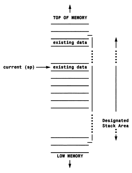
Before control is passed to a subroutine the processor calculates the address of the next instruction (ie the one which would have been executed if the subroutine call jump was not going to be made). As mentioned above, this address is placed on the 680x0’s stack so that as the jsr instruction passes control to the subroutine this is the state of the stack (Figure 4.3) overleaf.

680x0 stacks then grow downwards in memory and since the stack pointer always points to the last data item added to the stack this means that before adding new items you must first decrease the stack pointer by a number equivalent to the byte-size of the object being stored — this way it properly points to the locations to be used next. The jsr instruction therefore decreases the stack pointer by four, stores the return address, and then places the specified jump location into the processor’s program counter. Note that it is common, when placing data items onto the stack, to talk of pushing data onto the stack.
The main body of the subroutine will execute just like any other piece of code but the last instruction of the subroutine will be a rts, return-from subroutine, instruction. This causes the address at the top of the stack to be retrieved (popped or pulled are commonly used terms for this operation) and placed in the 680x0’s program counter. The result is simple. The processor jumps to the newly specified address and this of course is the return address specified during the original subroutine call.
A further instruction, called branch-to-subroutine (mnemonic bsr), provides a relative addressing form of the subroutine call mechanism. In this case either an 8 or 16 bit displacement can be provided. We briefly mentioned in Chapter Two that the 680x0 supports the use of separate supervisor and user stacks, which allows system software running in supervisor mode to maintain its own stack area. For the programs discussed in this book, whenever we talk about the 680x0 stack we are referring to the user-mode stack!
Push and Pull
There’s a point concerning the pushing and pulling of data from the stack that is worth clarifying. When data is placed on the stack it is, like all other 680x0 data movement operations, a copy of the data that is written into the stack area. Similarly when data is pulled from the stack it is a copy of the stack data that is retrieved. If, by way of example, we could see the state of the stack just after the subroutine being discussed earlier executed its rts instruction, Figure 4.4 illustrates what we would find.

Although a copy of the return address has been placed in the program counter and the stack pointer adjusted, the return address originally placed on the stack is still there. What of course happens is that the next time a subroutine call is made those locations get over-written with the new address!
Parameter Passing
The programs and code fragments that we’ve been looking at in the previous chapter are simple examples and not exactly typical of the code you’ll find in real programs. Most proper programs will need to perform a variety of tasks and many of these, because they either need to be done many times or because they concern jobs which are common to numerous programs, will be written as subroutines.
Apart from the fact that subroutines can save memory space there are other benefits. A subroutine that has been written to be generally useful will, after suitable preliminary testing, be able to be used by programmers secure in the knowledge that it is safe, ie the subroutine does what it is supposed to and is error free. In fact maximising the utility value of such routines is a good design objective because the more generally useful a piece of code is, the more the programmer will find uses for it. Similarly, maximising the use of either system supplied or self-written subroutines makes program development quicker and this re-use of tested code also reduces the chances of bugs. In fact you can almost guarantee that any bugs that do occur in your program will come from the code that you’ve written and not from the library subroutines being used.
Most of the subroutines that you’ll code in your own programs will use absolute or relative addressing simply because you will know the address of the routine at assembly time. You should be aware however that it is possible to devise extremely sophisticated subroutine access mechanisms using other 680x0 addressing modes. I briefly mention the possibility of hash-access and table access calls in Chapter Five and the Amiga’s multitasking Exec Kernel uses a dynamic library system built around loadable libraries of subroutines that are accessed indirectly. The Exec library system is in fact so important that I’ve devoted a whole chapter to it (see Chapter 10)!
You will incidentally see both the terms function and subroutine in much Amiga literature. In fact all of the library subroutines are called functions and this stems mainly from the fact that the C language (upon which the Amiga and its documentation is very dependent) calls all subroutine-like procedures, functions! In other non-C areas of computing one normally reserves the term function for a subroutine that acts on some data and returns a single result. A subroutine which takes the address of a text string and returns its length would be called a function, a subroutine which sorted a set of words into alphabetical order would not! Because you will find that almost all Amiga documentation will be using the term function you’ll find that, outside of this chapter, I will be doing the same when discussing Amiga system routines.
In order to be really useful, subroutines must be written so that they are general. There is, for instance, little point in writing a subroutine that prints the message Please enter a number! It would however be quite useful to create a subroutine that could print any text message specified by the main program. This brings us to one of the most interesting areas of subroutine use. Namely, how such information can be provided to the subroutine and how any results might be passed back. Data items that are to be passed to a subroutine are called parameters and the act of arranging to transfer these parameters to the subroutine is called parameter passing.
There are two basic ways in which data can be passed to a subroutine:
-
Parameters may be placed in the 680x0’s registers.
-
Parameters can be stored in memory
Register-Based Parameter Passing
This first option is both simple and fast. Since pointers to larger objects, such as strings and other blocks of data, can be passed, ie the subroutine can be passed the address of the object rather than the object itself, there is little you cannot do. Similarly the subroutine may return any results, or a pointer to those results, directly in a register.
Memory-Based Parameter Passing
The advantage of this option, despite the fact that it is usually slower, is that it offers more flexibility. Parameters can, for example, if they are known at assembly time, be placed in memory immediately after the subroutine call. For example:
                  .
                  .
                  jsr     SomeRoutine
  orig_rts        dc.l    #data_item1
                  dc.l    #data_item2
                  .
                  .
                  .
                  dc.l    #data_itemN
  needed_rts              remaining instructions
                  .
                  .
In this case the return address placed on the stack by the processor would be wrong — the 680x0 wouldn’t realise that the numbers immediately following the jsr call were data rather than a valid 680x0 instruction. In short the return address would need to be altered by the subroutine itself, by adding to the return address an amount equal to the number of bytes of parameters. Other approaches include the passing of a pointer to a parameter block in a similar fashion. An often simpler method is to use global variables, defined and labelled locations that can be read from any routine anywhere in the program.
None of these solutions provide sufficient generality to have found widespread favour but the next, stack-orientated, approach I want to discuss has. Although the 680x0 stack was introduced during the discussions of subroutines and return addresses it is now time to point out that the 680x0’s stack can be used for the storage of other data, namely bytes, words and long words. With the 68000 and 68010 processors word and long word, data must be word-aligned and the 680x0 stack pointer register does in fact take a special precaution to ensure this word alignment — it word-aligns all data, even single byte values. When byte data is pushed onto a 68000/68010 stack, it is stored in the high-order byte of a 16 bit word.
Stack-based parameter passing can be done by several means. The 680x0’s move instruction can, for example, be used in conjunction with indirect addressing with auto decrement to push a value onto the stack like this:
  .
  .
  .
  .
  move.w  tab_size,-(sp)  push tab size parameter
  jsr     ExpandTab       expand to spaces
  .
  .
  .
  end of program
What must be remembered of course is that, after you have pushed the parameter onto the stack, the jsr instruction will have subsequently pushed a return address so the stack will be looking something like Figure 4.5.

This means that the subroutine needs to look not just at the top of the stack but actually into it in order to see the parameter. Since the return address is four bytes long we have to use a displacement of 4 as this example shows:
  ExpandTab move.w 4(sp),d0       retrieve tab size in d0
          .
          .
          .
          rest of code            do something
          .
          .
          .
          rts
The above fragment copies into d0 the two bytes of data immediately above the return address. The situation once the subroutine has returned is that the stack pointer will, at least in the case of the current example, be left pointing to the parameter that we placed on the stack. This cannot be left because it will destroy the integrity of the stack as far as any items which have been placed on the stack earlier are concerned. The parameter is not needed and so there is little point in executing a move (sp)+,d0 type pull instruction. Instead the simplest idea is to numerically adjust the stack pointer so that the item is effectively ignored:
  .
  .
  .
  move.w  tab_size,-(sp)  push tab size parameter
  jsr     ExpandTab       expand to spaces
  addq.l  #2,sp           clean-up stack
  .
  .
  .
  end of program
The Amiga’s amiga.lib linker library routines use this type of mechanism and I’ll be looking at some real Amiga examples of this technique in Chapter 12.
Other stack-orientated instructions are available, including a very useful one called push-effective-address, which can both calculate an address using any of the 680x0’s addressing schemes and push it onto the stack for you. An example which shows the use of this instruction is given in Chapter 12.
Register Preservation Using Movem
Normally it is advisable to create subroutines which do not alter the contents of any temporary registers that they may use, ie those that will not be used to return a result. The best way to do this is to preserve those registers by pushing their contents onto the stack, restoring them just before the subroutine returns.
One way of doing this is to push/pull the contents of each register singly using instructions such as:
  move.l a6,-(sp)         preserve a6 on stack
  move.l a5,-(sp)         preserve a5 on stack
  move.l a4,-(sp)         preserve a4 on stack
                          do something

  move.l  (sp)+,a4        restore contents of a4
  move.l  (sp)+,a5        restore contents of a5
  move.l  (sp)+,a6        restore contents of a6
but in actual fact a special multiple move instruction exists, called movem, which allows this transfer to be done more efficiently when two or more registers are involved.
Movem actually exists in two forms. The instruction used when transferring registers to memory is called, not unsurprisingly, Move-Multiple-Registers-To-Memory (mnemonic movem). It can use all of the absolute and indirect addressing modes except the autoincrement mode. This is a deliberate restriction because it forces the programmer not to use to autoincrement when placing data on the stack (that approach would cause stacks to grow upwards in memory which would contradict the 680x0 stack conventions).
Its useful to look at how this instruction is designed internally. The first word contains bit patterns which identify the instruction, the transfer size, and the effective destination specification. The second word is a 16-bit mask which has been assigned to represent registers either in this fashion:
a7 a6 a5 a4 a3 a2 a1 a0 d7 d6 d5 d4 d3 d2 d1 d0or, if the automatic predecrement addressing mode has been specified, like this:
d0 d1 d2 d3 d4 d5 d6 d7 a0 a1 a2 a3 a4 a5 a6 a7Registers are moved in the order bit 0, bit 1, bit 2 etc, of the mask and so the order is d0, d1, d2 etc for the normal mask and a7, a6, a5 etc, for the reversed mask (assuming that is that the appropriate mask bits for those registers have been set to 1).
The equivalent Move-Multiple-Registers-From-Memory, movem, instruction does not use this mask reversal. In fact it always uses the bit mask arrangement described first, ie:
a7 a6 a5 a4 a3 a2 a1 a0 d7 d6 d5 d4 d3 d2 d1 d0and instead it allows the autoincrement addressing mode but does not allow the predecrement form.
When multiple data items are placed onto the stack the order in which they are removed is important. Because the stack works on a Last-In-First-Out arrangement items must be removed in the reverse order to that used to originally put them on the stack. If for instance you store registers d0, d1 and a1 (in that order) then to re-instate the registers you must first pull a1, then d1 and finally d0. The effect of the mask reversal scheme when using the predecrement form of the movem instruction is that this ordering reversal occurs automatically and the program doesn’t have to explicitly worry about it (the assembler generates the appropriate mask).
The easiest way to describe the use of the instruction is to show you some examples. To save on the stack the full 32 bit contents of registers d0 through d7 and a0 through a3 for example we would write:
movem.l d0-d7/a0-a3,-(sp)To restore the registers (ie pull them back off the stack) we’d use:
move.l (sp)+, d0-d7/a0-a3Similarly to preserve register d0 and registers a2-a5 we use this instruction:
move.l d0/a2-a5,-(sp)and to restore the contents:
move.l (sp)+, d0/a2-a5These instructions have a number of uses but as far as their use in subroutines is concerned you’ll mainly see them used on entry and just before exiting (ie just before the rts instruction) like this:
  SomeSubroutine  movem.l d0-d4/a0-a3, -(sp)      preserve registers
          <main body of subroutine code>          do something!
                  move.l  (sp)+, d0-d4/a0-a3      restore registers
                  rts                             return
When registers are preserved like this, routines which are expecting parameters to be passed on the stack need to allow for the fact that more items have been pushed onto the stack after the return address. In the above example nine 32 bit registers are preserved (d0, d1, d2, d3, d4, a0, a1, a2, and a3) so a further 36 bytes have been placed on the stack. If we go back to the stack-based ExpandTab parameter passing example mentioned earlier and add the above register preservation code, the offset now needed to access the tab size variable would be (9 x 4) + 4, ie 40, and the code would then be based on this type of framework:
  ExpandTab       movem.l d0-d4/a0-a3, -(sp)      preserve registers
                  move.w  40(sp),d0               retrieve tab size in d0
                  .
                  .
                  .
                  rest of code                    do something
                  .
                  .
                  move.l  (sp)+, d0-d4/a0-a3      restore registers
                  rts
Link/Unlk Instruction
More sophisticated subroutine arrangements are possible and one scheme used by many 680x0 based high-level language compilers (including C) is not only able to eliminate the need for the altered displacements illustrated in the previous example but provides a number of other benefits.
The idea is that as soon as a subroutine is entered we immediately preserve the contents of an address register on the stack and then copy the stack pointer into it. This then establishes that register as a fixed frame pointer which can be used to access any parameters lying above the frame pointer and return address. Having done that, it is then possible to decrease the real stack pointer (ie register a7) by some chosen value such that this amount of space is then available as temporary workspace on the stack. After this has been done the subroutine can do all its usual register preservation operations and data subsequently placed on the stack will be stored after (ie below) the temporary hole that we’ve created in the stack. If, for example, a5 was being used as the frame pointer register we’d end up with the situation shown in Figure 4.6 overleaf.

The situation in Figure 4.6 is then that after the frame pointer has been set up (a5) + 8, in other words the contents of register a5 plus an 8 byte displacement (remember that the return address and the frame pointer are both stored on the stack at this time), identifies the start of the parameters (if any) that are present on the stack. Another benefit of this arrangement is that by using negative displacements it becomes possible to access the temporary stack workspace, which was created when we made a hole in the stack by decreasing the stack pointer. In a high-level language it is just these kinds of negative displacements that are used to create local variables, which exist only during the execution lifetime of the routine in question.
Best of all though is the fact that the real stack pointer is set to the low end of our temporary workspace so, even when any number of new items are pushed onto the stack, the frame pointer remains valid.

At the end of the subroutine any additional items placed on the stack by the routine are removed and then the stack pointer is advanced past the work area, by loading it with the contents of the frame pointer. The original frame pointer register contents are then pulled off the stack and placed in the register used as a frame pointer, so re-instating it to its original value, and a normal subroutine rts is performed. This latter instruction, as usual, removes the return address placed on the stack by the jsr (or bsr) instruction.
OK, there are some difficult things to grasp with this approach but the general outline and power of the technique should be apparent. What you might like to know however is that the 680x0 provides two instructions which allow this complex set of operations to be done automatically. The instructions are called link and unlink (mnemonic is unlk) and they are used like this:
  MySub   link    a5, -32                 create 32 byte work area
          movem.l d0-d7/a0-a2, -(sp)      preserve some registers
    main body of the                      providing it is not
    subroutine will use                   destroyed by the sub
    (a5) displacements                    routine itself a5
    to access parameters                  remains valid no matter
    and local workspace                   what happens to the
                                          stack pointer
          movem.l (sp)+, d0-d7/a0-a2      restore registers
          unlk a5
          rts
The link/unlk instructions can dynamically allocate up to 32768 bytes of stack workspace, and as you’ll see from the example the workspace displacement size needs to be given as a negative number, because the stack is growing downwards.
If, incidentally, you ever disassemble compiler generated code you will see link/unlk instructions being used to preserve space for local variables. In fact an interesting example of this type of use is provided later in the book!
Styles and Subroutines
There are characteristics of some subroutines which, although they will not be particularly important or relevant to the assembler newcomer, are worth briefly mentioning since the terms do crop up in the Amiga official documentation from time to time.
Truly relocatable routines are routines that may be placed anywhere in memory. They are created by using relative addressing instructions so that absolute memory references are avoided. You might think that, because of the way the Amiga loads its programs and data into any convenient spare memory that is available, that all Amiga programs would need to be relocatable. This isn’t true because the Amiga uses a piece of program loading software called a relocating loader which is able to take a program containing absolute address references and modify them (ie add a loader calculated offset) so that the program runs properly at the chosen location.
Re-entrant routines are routines that may be interrupted, called by the routine which did the interrupting, and still produce the right results. This allows interrupt system code to make use of available system routines.
Recursive subroutines are routines which are able to call themselves during the course of their operations. Subroutines which preserve their registers and use only those registers and the stack for storing data will be capable of being used recursively. Needless to say they will also be re-entrant!
Subroutines on the Amiga are very important and, as mentioned earlier, the Amiga’s run-time and link-time function libraries contain a great many pre-written subroutines for you to use. It is no exaggeration to say that upwards of 80% of the assembly language code that the average Amiga assembler programmer will write will be library related and consist of calling pre-written functions to do particular jobs. To a large extent your coding efforts will just revolve around making sure that your program performs the necessary library routines in the right order and with the right types of integrity checks.
In many ways the use of pre-written routines can be alikened to using a piece of hardware like a photocopier. If you use a photocopier to make a duplicate of something you go to the machine, place the document you wish to copy inside, press a button, and then just wait for the device to do its job. As likely as not you’ll do all this without knowing any real details about what goes on inside. In a sense the copier is acting almost like a magic black box. You know what input is required (the document to be copied), what must be done to start the copying process, and you know that some results will come back, ie you’ll get a copy of the input document.
This information hiding, black box, design concept is a very powerful way of protecting a user from unnecessary complexity. For the programmer, the pre-written subroutine unit provides exactly the same type of complexity hiding capabilities and, on the Amiga at least, constitute essential program building blocks to be used in the same way as the electrical engineer might use IC chips (integrated circuits pre-designed to do a particular job) to build an electronic circuit.
There is one general point about this pathway which is important. Although the user of the function doesn’t need to know how the subroutine works, they do need to know what it does, what information must be supplied, and the significance of the results produced, this means that the user must have suitable documentation for the system routines. This of course is one of the reasons that books such as the RKM Includes & Autodocs manual, which lists function usage descriptions for all of the Amiga’s library functions, are so important.
5. Program Design Issues
This book is not about program design but there is no doubt that programming a machine as complex as the Amiga is almost impossible unless you adopt some kind of forward planning. That for most people means taking more than a passing interest in the techniques used for program design. I’m not going to review the many tools which are available but I am going to provide some examples of a method that I have found to be of immense value with all kinds of programming, including 68000 assembler.
It’s based on a logic design tool called the Warnier diagram and, before looking in detail at the ideas involved, I want to make the following point. The methods I am about to discuss aim to obtain solutions to problems that are completely independent of both the computers and the languages which might eventually be used to implement the chosen design. These latter factors may well affect the final coding stages, but they should not usually influence the overall layout of the design.
So, what is a Warnier diagram? Essentially it is a set of curly brackets, that define both particular groups of operations and the order in which they should be performed. The easiest way to show you about these diagrams is to take some examples and I’ll start by taking one which will let me explain some important diagram conventions.
Imagine we wish to produce a report, consisting of details held on a computer file on disk. The Warnier diagram of the basic problem is shown in Figure 5.1 (over).

The bracket is read from top to bottom and describes a procedure or group of operations that has, arbitrarily, been called REPORT. The numbers which you see written underneath the various statements identify how many times the item is to be performed and, with just those two conventions, our first diagram is already illustrating some of the essential features of the problem.
Do we know anything more about the problem? Can we think of any information that could be relevant? Well, we know that computer files need to be opened before reading and closed once the read operation is complete. These details could therefore also be added to the diagram. To enable us to explain some further conventions used with Warnier diagrams let us first add a minor complication to the problem. Let us suppose that the user wishes to access a file of his (or her) own choosing and to obtain a printed report of the details on the file. The specified file may not exist, and, if this is the case, the user should be informed. These changed or altered requirements can be represented by a more detailed Warnier diagram.

Figure 5.2 shows, in Warnier diagram form, the requirements of the problem as it is at the moment. We are using the convention that the logical opposite of a statement is written by placing a bar over it.
  ___________
  FILE EXISTS means FILE DOES NOT EXIST
We are also using a (+) sign to separate mutually exclusive operations (sets of operations which will not occur together). In the present example the file will either exist or it will not exist, so only one of these two operations would be performed at any one time and (0,1 time) is written underneath the statements involved. At other times the operations shown within a bracket may need to be repeated and in these cases an expression such as (1,N times) would be used.
The conventions used so far are in fact the only ones you will need for the majority of problems that you are likely to encounter. Here they are collected together for convenience:
-
Brackets are used to define sets of operations.
-
Brackets are read, and performed, downwards within any one level. The item at the top of the bracket is performed first, the item at the bottom performed last.
-
The logical opposite of a statement can be written as the original statement with a bar drawn over it.
-
Brackets written to the right of a statement indicate the operations to be performed if that statement is performed.
-
Underneath each item or statement we indicate the number of times the operations should be performed.
-
Mutually exclusive statements are written separated by a (+) sign.
Using these conventions we can express in English exactly what Figure 5.2 tells us: we are dealing with a certain procedure, called REPORT that starts by asking for the name of a file. If the file exists then it is opened, accessed, the details printed, and then the file is closed. If it does not exist then the operator is informed of the fact. Remember that if the file does exist then it is the group of actions (subset) shown to the right of the label FILE EXISTS that are performed.
To appreciate the elegance and speed with which these diagrams can accommodate changing requirements let us place some further restrictions on this problem. Within this hypothetical computer system are files containing sensitive data, perhaps personnel data, wages or medical records. Such data must be protected from unauthorised access and users are therefore issued with access code numbers, so that examination of sensitive files is restricted to those users with the proper authority. If unauthorised attempts to access this data are made the computer should record the fact, perhaps by making an entry into a special security file.

Let us first consider the new constraints in isolation. We need to check whether the file specified by the user is a restricted file, if it is we must ask for the user’s code number. If the code is correct then we allow access, if not we write a security record indicating an attempted illegal access.
The diagram in Figure 5.3 shows the Warnier form of our new requirements. Notice that as we redefine the problem and add more detailed restrictions it is not necessary to rearrange the complete diagram, as one frequently needs to with flowcharts etc. All we have to do is superimpose the new details and restrictions on to the existing diagram structure. The diagram is therefore actually growing as we successively modify and redefine the known details of the problem. You’ll see later that the Warnier diagram is not only documenting and expressing the logical requirements of the problem but it is doing so in a way that will make the transition to a computer language equivalent form remarkably simple.
The ability of the Warnier diagram to display, help formulate, and to grow with the changing logical requirements of a problem, as that problem is examined, is of great importance. Once the quite simple conventions have been learnt these diagrams can be read just like the written English equivalent but, unlike the written English form, a Warnier diagram contains within its deceptively simple notation, the complete solution to the coding of the problem.
The secret of converting a Warnier diagram into a finished program lies in regarding each bracket involving more than one operation as a subroutine. There are certain exceptions to this general statement but the pseudo-BASIC sketch shown in Figure 5.4. should give you the general idea.
A Second Example
For this second example, which again is a general, rather than an Amiga specific illustration, I’m going to design the basic structure of a routine that collects characters from a keyboard device. If the character is a carriage return (ie ASCII 13) then the routine should terminate, if it is another control character then an appropriate control character subroutine should be performed. If the character is not a control character then it should be passed to a printing routine to display it on a VDU or other output device.
  * ======================================================

   P S E D U O - B A S I C - R E P O R T - M O D U L E

  *

  INPUT NAME OF FILE

  IF FILE EXISTS THEN GOSUB `FILE EXISTS' ELSE PRINT `FILE DOES NOT EXIST'

  RETURN TO CALLING PROGRAM

  *

  REM SUBROUTINE..........FILE EXISTS

  IF FILE IS RESTRICTED THEN GOSUB `RESTRICTED FILE' ELSE GOSUB `ACCESS'

  RETURN

  *

  REM SUBROUTINE..........RESTRICTED FILE

  INPUT SECURITY CODE

  IF SECURITY CODE=CORRECT CODE THEN GOSUB `ACCESS' ELSE GOSUB `ILLEGAL ACCESS'

  RETURN

  *

  REM SUBROUTINE..........ILLEGAL ACCESS

  WRITE TO I/A LOG FILE THE TIME OF ATTEMPT AND THE ACCESS CODE

  PRINT `THIS IS A RESTRICTED FILE - PLEASE MAKE NO FURTHER ATTEMPTS'

  RETURN

  *

  REM SUBROUTINE..........ACCESS

  THIS WOULD BE A ROUTINE TO ACCESS THE DATA IN THE FILE AND DISPLAY ON TERMINAL OR PRINTER ETC.

  RETURN
* ======================================================Let’s first quantify what’s known about the problem in terms of the sort of operations which might be needed. We will have to input a character, possibly using an input routine available within the operating system. Some type of check will also need to be made to see whether an input character corresponds to a control character or not. For the purposes of the example we’ll regard a control character as one with an ASCII value of less than decimal 32. Additionally some means of printing characters is needed but since such facilities are usually provided by the operating system we’ll assume that such a routine is already available.
The first step is to create a Warnier diagram sketch showing those objectives which are relatively obvious from the original statement of the problem.

Figure 5.5 shows a first attempt at describing the problem. The diagram implies that a test can be performed which will indicate whether a given input character is a carriage return or not. Additionally it implies that a character can be tested to see if it is a control character. We should be fairly happy with this initial diagram because all general computer languages, both high and low level, provide the type of testing needed to perform the necessary tests.

At present the Warnier diagram does not indicate that we collect anything more than one character by performing the illustrated operations. It is necessary in practice to perform the operations in Figure 5.5 any number of times from 1 to N times, depending on when the user supplies a carriage return character.
Figure 5.6 (above) explicitly shows that we perform the operations indicated in Figure 5.5 at least once, and up to a maximum of N times. The labels used are, of course, arbitrary, but it is obviously advisable to choose meaningful English expressions since this enables the diagrams to be more easily understood.
Now that a reasonably accurate representation of the problem is available it’s time to consider some more detailed requirements: Let us suppose that the control characters detected are going to be used to perform the operations shown in Table 5.1 below.
        ASCII code      Operation to be performed
        8               Move cursor to left.
        16              Move cursor to right.
        10              Perform a line feed.
        9               Perform a tab.
        11              Move cursor down.
        12              Move cursor up.
        Others          Take no action (ie ignore them all).
These operations are a more complex example of the mutually exclusive operation sets mentioned earlier. Notice that in this case the bar notation cannot be used because many alternatives exist. Instead the options are written using their respective names (separated of course by the (+) sign to indicate that each operation subset is mutually exclusive). Figure 5.7 shows how this situation is represented in Warnier diagram form.

Let us now make an alteration to the control character routine by creating some further assumptions. We suppose that if our hypothetical user presses a control key that serves no apparent purpose then either a simple error has been made (the user has pressed the wrong key) or the user is under the impression that the control key pressed serves some function which it does not, in fact, perform. In either case we may, from a practical point of view, decide to provide some means of informing our user that a useless or unsupported key has been pressed.
I’ll assume, since this is a general example, that the VDU screen has either one or two lines available for comments or for collecting responses such as input from the user, or that some type of requester/dialogue boxes are available for these types of simple I/O operations. The implication here then is that most of the screen contains information that must be preserved, so we cannot simply print a menu of control character options on to the screen.
Nowadays of course on machines like the Amiga it is the WIMP (Window, Icon, Mouse, Pull-down menu) system that would handle the screen preservation actions, but for the purposes of this example let’s assume that it is the applications program itself that must take all necessary actions.
As far as the example is concerned then we will need both space on the screen to display a menu, and somewhere to save the existing contents of the VDU screen. It might also be useful to ascertain whether the user actually needs a menu. Perhaps he or she will often quickly realise that a wrong key has been pressed by mistake and just want some way of getting back to normal operations as quickly as possible.
To tackle this new set of problems it is useful to first consider the new restrictions as a discrete subset of operations, ie concentrate on just the new requirements. Once a suitably structured diagram concerning the new constraints has been created it can then be superimposed onto the original diagram in Figure 5.7.

The diagram in Figure 5.8 shows our latest requirements in Warnier diagram form. Convince yourself that the known additional details have been expressed in a suitable manner, then look at Figure 5.9 which shows the whole of the control character description including the latest additions.

I could continue to expand other statements to provide further detailed analysis of the problem. As we do so we reach a point where it is possible to say: Yes, the operations we are describing in the lower levels of the diagrams (the right-most levels) are easily capable of being coded directly in the language I have chosen to use! In practice we reach this point far sooner with high-level languages than with assembly languages because more complex operations are supported.
The relevant point to make is that the general principles are the same. The only difference is that when you analyse problems that will be coded in assembly language you will need to carry the analysis further.
In the illustrations given the Warnier diagram was used basically as a tool for expressing, and documenting, ideas and thoughts. The finished design was therefore achieved by a process of iterative refinement. There is nothing fundamentally wrong with this approach, even though in practice ideas are likely to change during the time that the initial Warnier diagram sketches are prepared. Very often it is the fact that you can represent your ideas in a pictorial fashion that will help you discover anomalies, faults etc. It is however possible to create Warnier diagrams directly using various logic devices such as truth tables, Karnaugh maps etc, and to check that a diagram is correct mathematically. This book is obviously not, however, the place for such discussions.
The 68000 Connection
You will doubtless have realised that in creating a Warnier diagram we are to a large extent planning the program control structure of the piece of software being designed. Consequently conversion to 68000 code revolves essentially around program control structure issues and there are a few points which are worth making about the 68000’s instruction set and the various instructions which can be used for creating the necessary control units.
Branches and Jumps
The 68000 as you know has two basic goto-like ways of transferring control. The jmp instruction which uses a full sized address, and the bra instruction which uses relative addressing based on a 16 bit displacement. In addition to this there are conditional branch instructions, which take the general form bcc and dbcc, that are able to perform relative branching when specified conditions are met or not met (branch on zero, branch on plus and so on).
The 68000 also supports two basic subroutine type instructions: The branch to subroutine bsr instruction is the relative addressing form of bra which additionally places a return address on the stack allowing a terminal rts instruction to transfer control back to the instruction immediately after the one that caused the subroutine branch in the first place. The second subroutine instruction of interest is the jump to subroutine jsr form which, like jmp, uses a full sized address rather than a displacement, jsr works like a jmp instruction but like bsr it places a return address on the stack.
In the context of usage flexibility there is a very important difference between the relative branching bra type instructions and full address orientated jmp and jsr forms. The latter instructions have much more scope in terms of available addressing modes. In fact there are seven addressing forms listed as being available for the jmp and jsr instructions:
-
Register Indirect
-
Register Indirect with Displacement
-
Register Indirect with Index
-
Absolute Short
-
Absolute Long
-
PC Relative with Displacement
-
PC Relative with Index
The indirect addressing modes are particularly useful for creating some of the more complex control structures. The instruction:
jsr (a5)for instance, performs a subroutine call to a location whose address has been placed in address register a5. The 68000 also has a load effective address lea instruction which can compute and load an address register with an address computed using any of the 68000’s addressing modes. This means that even with the simple indirect subroutine call the processor can be instructed to perform an infinite number of complex subroutine call arrangements. The first instruction of the following fragment, for example, takes an address held in register a2, adds it to the value held in register d4, and then adds a program-specified fixed offset (12 hex in the example) to produce an operand address which is then loaded into register a5. The second instruction performs a subroutine jump to that calculated address:
  lea $12 (a2, d4.l) a5
  jsr (a5)
Not only does this mean that we’ve got very flexible conventional run-time (dynamic) and static address calculation facilities but also that things like key-to-address transformation (hash based) schemes are also relatively easily built:
  jsr     CalculateAddress        calculate hash address in d0
  move.l  d0,a5                   copy to a5
  jsr     (a5)                    call appropriate subroutine
The net result of all this is simple: the 68000 itself is not likely to place any restrictions on what you can do control-wise because all manner of clever schemes can be devised. In fact once you start working at the processor level you begin to realise that the addressing modes of the 68000, coupled to its relatively symmetrical instruction set, actually tends to liberate, rather then restrict the programmer. At times I sometimes wonder whether it isn’t the high-level languages which suffer from shortcomings rather than the low-level ones although I’m sure most people would disagree.
The point again needs to be made that one of the reasons that I feel just as comfortable working with assembly languages as with high-level languages is that before I write one line of assembler code I’ll have a logical plan available which shows what must be done!
Black Boxes
I’ve made quite a point elsewhere of talking about information hiding and black box units, subprogram/subroutine units. The ability to create isolated pieces of code which can be used without knowing how they operate makes for re-useable and easily modifiable code units. Inherent in such ideas of modular program construction come two other needs: decent parameter passing schemes as opposed to routines which use a hotchpotch of globally accessible memory locations, and the ability of a routine to create and use variables which are known only to them. Languages like C provide inbuilt mechanisms for parameter passing and use of local variables, but how can we do it from assembler?
There are a number of schemes but one, stack-based allocation, stands out as being particularly important. The idea is simple. As a subroutine is entered the stack pointer register is altered so that some temporary working space is preserved on the stack for the variables and other quantities needed by the routine, conveniently accessed by setting up a frame pointer which allows the workspace to be accessed indirectly. The 68000 has a powerful instruction pair called link/unlk which allows this whole process to be automated.
Another important technique, which we’ve already discussed, is that of preserving and re-instating processor registers during subroutine calls. At the start of the routine you preserve, by pushing onto the stack, those registers which are going to be utilised during the subroutine call. Just before the routine terminates the pushed values are pulled off the stack and used to return the processor to its original state.
For now though, with the above preliminaries out of the way, it’s time to look at some of the basic ways in which the sequence, repetition and alternation building blocks can be tackled with 68000 assembler.
Control Constructs — Sequence
As you might expect, sequence is the easy one. Sequence is implied simply by virtue of the order in which statements are written. If, for example, you need to code something like this:

then, if all the operations were going to be handled as subroutines, you might write something along the lines of:
  jsr InitializeReplyString
  jsr CollectResponse
  jsr InterpretReply
of course if one or more of the operations were simply enough, ie consisted of just a few relatively obvious instructions, then they might be coded in line.
Suppose that the above routine was using a0 as a reply string pointer and that the strings were using the NULL terminator convention. To initialize a string in such a situation all that needs to be done is to set the first byte (which would be the byte represented by the address held in a0) to NULL, so the above example would just as likely be coded as:
  move.b  #NULL,(a0) initialize reply string to ""
  jsr     CollectResponse
  jsr     InterpretResponse
Similarly if you were using some system routine to collect a user string and this routine needed to have the start of the string supplied in d0 you might have a fragment like this:

In such a case it’s not hard to see the sort of translation that would be needed:
  move.b  #NULL,(a0)      initialize reply string to ""
  move.l  a0, d0          system requires start address in d0
  jsr     CollectResponse
  jsr     InterpretResponse
Control Constructs — Repetition
Consider the following fragment:

Repetitive sets, when coded, end up as loops. If we choose register d0 as a loop variable then the obvious way of coding the above fragment would be along the lines of:
        move.b  #L00PC0UNT, d0
  Loop  jsr     GetCharacter
        subq.b  #1,d0
        bne     Loop
Of course the 68000 has an automated loop instruction dbcc which handles both the counter modification and, if needed, an extra conditional exit test. Bearing in mind that dbcc quits the loop when the counter register hits -1 (so the count must start at one less than the required value) we’d probably write the above loop like this:
        move.b  #LOOPCOUNT-1, d0
  Loop  jsr     GetCharacter
        dbra    d0, Loop
If the extent of the repetition is not known in advance, as in the now wellworn case of collecting keyboard characters until such time as a return key is detected, then we modify the test conditions accordingly. Supposing that in the above example the GetCharacter routine, as well as placing the collected character into a string buffer, also returned the
        jsr     GetCharacter
  Loop  cmp.b   #CR,d0
        bne     Loop
At times you might wish to show the exit conditions explicitly on your Warnier diagrams. The fragment for the above example might therefore have been written as:

It is not worth being pedantic over the form, or the notation, for such translations. If a repetitive loop requires an exit condition which is obvious to code then there is little point in cluttering up the Warnier diagram with unnecessary detail. Having said that there is, for documentation purposes at least, a case for including some note about any tests which are implied rather than explicitly diagrammed. Bracketed comments do nicely here:

The bottom line then is simple: you take your diagram detail to the point where the actions being specified become easy to code. Obviously the point where this occurs will vary according to your programming abilities and the problem being dealt with! The above loops are post-test forms — the exit condition occurs at the end of the loop. Pre-test repetition, ie repetition of the while/wend variety, is just as easy to create. Take the following diagram fragment:

If we assume that a0 holds the address of the first byte of the string being dealt with, we might code the above fragment like this:
    cmp.b   #NULL,(a0)        is first byte a NULL?
    beq     Here
    jsr     ConvertToLowerCase
  Here
The implication here is that if the string is empty, ie contains only a terminal NULL character, then the ConvertToLowerCase routine is never executed. It’s interesting to note, but I’m not going to dwell on this, that the assembly language form actually shows the fundamental nature of the repetitive set which occurs one or more times. The above code actually represents this situation:

Control Constructs — Simple Alternation
To be honest we’ve already started looking at alternation in the sense of loop termination testing. The if-else type testing needed for fragments like:

can be coded using these type of schemes:
          jsr     CheckPrinter    z flag indicates connection Print
          beq     Print
          jsr     PrinterMessage
          bra     Here
  Print   JSR     PrintFile
  Here
Control Constructs — Case Alternation
It is possible to extend the above simple alternation schemes to cater for case alternation. This leads to a step by step evaluation of each case. For example:

Could be coded using this type of framework:
  LinefeedTest            cmp.b   #LINEFEED,d0
                          bne     CarriageReturnTest
                          ;do line feed related stuff
                          bra     CaseEnd

  CarriageReturnTest      cmp.b   #CARRIAGE_RETURN,d0
                          bne     TabTest
                          ;do carriage return related stuff
                          bra     CaseEnd

  TabTest                 cmp.b   #TAB,d0
                          bne     BackspaceTest
                          ;do tab related stuff
                          bra     CaseEnd

  BackspaceTest           cmp.b   #BACKSPACE,d0
                          bne     OtherCharactersTest
                          ;do backspace related stuff
                          bra     CaseEnd
  OtherCharactersTest     ignore or do whatever else is necessary

  CaseEnd...
Whether the individual actions associated with each case get written as subroutines calls, instead of being written in line, depends to a large extent on what is involved. If you are happy that the necessary code details are easily handled then by all means place them in line. Here’s an example. Suppose that the fragment we’ve just discussed had to expand tab characters to spaces. The relevant details might have been diagrammed as:

The general type of loop for such space insertion would therefore go something like this:
                  move.b  g_tab_count,d1  get conversion count
  InsertSpace     move.b  #SPACE,(a0)     insert space
                  addq.l  #1,a1           move to next character
                  subq.b  #1,d1           decrease count
                  bne     InsertSpace
Using post-increment addressing and the specialised dbcc instruction, the above loop can be written more concisely as:
                  move.b  g_tab_count,d1  get conversion count
  InsertSpace     move.b  #SPACE,(a0)+    insert space/increment a0
                  dbra    d1,InsertSpace
There would be no problem in coding those three lines directly. Most assembly language programmers would be able to fill that TAB segment so that the skeleton code framework then looked something like this:
  LinefeedTest            cmp.b   #LINEFEED,d0
                          bne     CarriageReturnTest
                          ;do line feed related stuff
                          bra     CaseEnd

  CarriageReturnTest      cmp.b   #CARRIAGE_RETURN,d0
                          bne     TabTest
                          ;do carriage return related stuff
                          bra     CaseEnd

  TabTest                 cmp.b   #TAB,d0
                          bne     BackspaceTest
                          move.b  g_tab_count,d1  get conversion count

  InsertSpace             move.b  #SPACE,(a0)+    insert space/increment a0
                          dbra    d1,InsertSpace
                          bra     CaseEnd

  BackspaceTest           cmp.b   #BACKSPACE,d0
                          bne     OtherCharactersTest
                          ;do backspace related stuff
                          bra     CaseEnd

  OtherCharactersTest     ignore or do whatever else is necessary

  CaseEnd...
The key, as always, is to only code those aspects which to you seem crystal clear. If you’re having trouble figuring out what sort of code should be written for a particular piece of diagram then the chances are that you’ve not taken the diagram to a sufficient level of detail. The solution is simple — expand your diagrams until they do represent that required detail.
Alternative Schemes for Case Construction
It must be said that, although the above approach has the advantage of being simple, there are occasions when it is inappropriate. One example which springs to mind is where a very large number of individual cases need to be catered for — if, for instance, you have a hundred different cases the above arrangement would lead (on average) to each character being tested fifty times. If you need fast case testing then the above approach is not going to help and alternative schemes need to be found. Here much depends on the particular application but if the values of the case structure entries are close together an indirection table, which provides the addresses of all of the case entries, can be used. You could, for instance, set up a table of routines like this:
INDIRECTION_TABLE:      dc.l Sub1, Sub2, Sub3, Sub4, Sub5,
                        dc.l Sub6, Sub7, Sub8...

Sub1:           some relevant code
                rts
Sub2:           some relevant code
                rts
Sub3:           some relevant code
                rts
Sub4:           some relevant code
                rts
Sub5:           some relevant code
                rts
Sub6:           some relevant code
                rts
Sub7:           some relevant code
                rts
Sub8:           some relevant code
                rts
etc...
It’s then possible to index the appropriate address locations and use an indirect subroutine call to select the appropriate piece of code:
  move.l  #INDIRECTION_TABLE,a5   base address (assume that the case data
                                  is in d0 so d0 times 4 will be the
                                  required table offset)

  asl.l   #2, d0                  multiply by 4
  move.l  (a5,d0.l), a0
  jsr     (a0)
If it were necessary to transfer control to some place other than the place after the subroutine call you could modify the above scheme by pushing your own return address onto the stack and then follow this with the equivalent jump instruction:
     move.l  #INDIRECTI0N_TABLE,a5   base address (again assume that the case
                                     data is in d0)
     asl.l   #2,d0                   multiply by 4
     move.l  #EndCase,-(a7)          push return address
     move.l  (a5,d0.l),a0
     jmp     (a0)
  ;(some other code or data, perhaps the indirection table itself, that shouldn’t be executed)
  EndCase...      continue execution at this point.
Design Summary
The overall diagram<->code conversion strategy should now be pretty clear. Having described the structure of the program using a Warnier diagram (or set of such diagrams) the conversion proceeds primarily by coding the various bracket levels as subroutines, only adding suitably detailed in-line instructions when the operations being dealt with are straightforward.
The reason why this approach is so effective is simple: It’s because most (if not all) of the design issues, as far as program structure is concerned, will have been dealt with before any coding is done. Consequently you’ll never at this stage have to ask questions like “whereabouts in the overall program should this piece of code be placed?”, or “what happens if this routine receives a character other than the ones it expects to receive?”.
I mentioned earlier that, as far as this type of diagram use is concerned the design process is iterative. This begs the question: when do you know that a diagram is finished? The answer is that you know that a diagram is finished when you look at the lower, ie most detailed, diagram levels and think: “Hey this isn’t so bad. All those things look easy to code!”.
I certainly do not get such translations right every time, neither does anyone else, and incidentally neither will you, no matter what design techniques you choose to adopt. Fortunately you’ll know when you haven’t provided a sufficiently detailed plan — all of a sudden you’ll hit coding difficulties because you are not quite sure of what you are doing. That of course is the time to stop coding, go back to your design diagrams, and think, preferably in a language-independent way, about what you are trying to do.
I will not be emphasising the pre-code design issues elsewhere in this book and certainly am not going to force you to adopt the use of Warnier diagrams. What I do want to drive home though is this: these pre-coding design issues, as any professional programmer will tell you, really are very important. Some knowledge and experience of either Warnier diagrams or some equivalent technique will make your life as a 68000 coder considerably easier!
6. Program Documentation
Over the years much has been written about the quality of program documentation and in the professional, large-project, arena there are many easily-enforceable guidelines for both user and system documentation. With smaller programs it is usually convenient to adopt a more flexible framework and so I’ll restrict my remarks to program comments which occur within the source code.
In-line comments, that is comments placed within the source code itself, should be a valuable documentation aid. Having said that, it is unfortunately not uncommon to find examples of program comments which are at best inadequate and at worst even misleading.
Such documentation failings can be serious for several reasons. Firstly, for better or worse, in-line program remarks tend to be long-lived. By their very nature they remain embedded within the code for the duration of its lifetime. Sometimes, even at a professional level, in-line comments may be the only form of program documentation available and if the comments are out-of-date, uninformative, or perhaps downright misleading then the maintenance of the program is likely to prove more difficult than if the program had been left uncommented.
In-line commenting problems fall into a number of recognisable classes:
-
Relatively pointless additions which essentially duplicate information that is obvious from looking at the code itself.
-
Comments which are misleading or incorrect.
-
Situations where so many comments are present that the important ones become hidden amongst a mass of trivial remarks.
-
Situations where an insufficient number of comments have been included.
-
Situations whereby comments have become dangerous by virtue of the fact that they are out-of-date.
Pointless additions are surprisingly common. A programmer may add a comment which simply duplicates something that is perfectly obvious from the code itself. For example:
move.l #0, count set count to zero!These types of additions arise for a number of reasons. Occasionally the less experienced programmer may include such a remark to remind themselves what they are doing. It’s an understandable trait but more experienced programmers reading the code will find such comments of no value whatsoever. There are however occasions where it might be necessary to draw attention to the fact that such an initialisation is important. This example for instance tells the programmer reading the code something very important about the variable in question:
  move.l #0, count        ;don’t forget that this count
                          ;variable must be set to zero each
                          ;time this routine is entered!
You will of course find a lot of comments in this book which, once you have some 68000 coding experience under your belt, will be recognised as stating the obvious. Such comments have of course been added to ease your passage through the code in the early days!
Comments which are misleading or incorrect can also be particularly troublesome. Programmers examining your program code will invariably accept in-line comments without question and this assumption, that any comments present correctly reflect the actions of the source code, is known to lead to the programmer suffering psychological blind spots. The results? Programmers may fail to recognise errors that might otherwise have been patently obvious.
Over-commenting is perhaps less of a danger but it is worth bearing in mind that rather more sparing use of comments in general might enable you to effectively highlight any difficult areas by providing additional comments in those areas needing special attention. This potential benefit is lost if such areas are buried deep within large numbers of less important comments.
A total lack of comments isn’t a danger, but it’s a nuisance because you have to work harder to understand what the program is doing if you wish to change something. There are a number of reasons why a programmer might not bother to comment a program. Perhaps the program was originally written for a once-only use, perhaps the programmer thought that the code was self-explanatory. Many programmers do not bother to change comments when they make program modifications. The result, another danger, is that program code and in-line documentation diverge.
Don’t make the mistake of thinking that comments are just to help other users and that you understand your code well enough not to need additional remarks. That may be so when you write the program, but you’ll be in for a surprise when you regularly start looking back at code you wrote several years ago — it’s amazing how code tricks which seemed perfectly obvious at the time seem to loose their inherent obviousness with the passage of time. The solution? Make sure that you provide decent in-line documentation and, most importantly, get the appropriate notes into the source code whilst you are creating the program — don’t wait until after the program is complete!
Several options exist for improving the quality of source code documentation. Comments should be structured in the same way as the program code itself. Remarks placed within a routine should be such that they apply only to the routine in question, not to the application which it is part of. This ensures that when a routine is re-used in another application, extraneous comments relating to a previous application are not inadvertently included.
Adopting a clean, structured, approach to program design helps to ease potential maintenance and commenting problems. Modules and routines should be created which communicate via well-defined interfaces so that the details of a particular routine can be hidden within that routine. Modules should be given comment headers which explain their purpose. At lower levels subroutines and functions should also contain details which provide an overview of the routines themselves, explain any conventions in use, identify the parameters expected, and indicate the way in which results are returned.
Self Commenting Languages
In-line commenting, whilst important, should still be considered essentially as an addition to, and not a replacement for, any self-documenting facilities of the language itself. Self-documenting facilities? Yes, nowadays almost all languages allow useful conventions to be adopted which can help to make the source code more intelligible and 68000 assembler is no exception.
Use understandable names for variables and symbolic constants. Adopt conventions such as prefixing global variables with the character g_ and suffixing pointer variables using _p, so that the type of variable can be implied from its name:
  move.l #FALSE, g_exit_flag      ;clear exit flag – user
                                  ;has decided not to quit
is a much preferred alternative to code which reads like this:
  move.l #0, ef                   ;clear global exit flag
                                  ;- user has decided not to quit
Don’t get carried away with such conventions. You are after all aiming to produce guidelines which can help, not build rigid restrictions which will hinder. For the most part all that’s needed is a common-sense understanding of the usefulness of in-line documentation, coupled to a consistent methodical approach. A bit of thoughtfulness in these areas will pay handsome dividends.
Guidelines
Before leaving the topics of languages, documentation and so forth there’s one last point to make. Whatever conventions you adopt you will need more documentation than any language alone can provide. Programmers are of course more noted for their Let’s do some coding attitudes than for any excessive desire to document their programs. But eventually failure to keep adequate notes will cost dearly, both in lessons not learnt and in lost time. The following guidelines provide a reasonable starting point although I’m sure that you are not going to be short of your own ideas:
-
The golden rule is simple. Document whilst you are developing the program and not afterwards. By all means tidy up the development notes after the program is complete but don’t wait this long before you make any notes at all. In this respect design techniques based on Warnier diagrams provide their own documentation as far as the progress of the design path goes. You’ll usually need however to keep plenty of other notes as well.
-
If possible try to develop a pseudo-standard layout for all your projects. Produce development notes that, in conjunction with any design work, will show what the objectives of writing the program were, and explain the reasons behind your approach. The task of producing this documentation is not quite as onerous as it might seem. If you have a text editor program then you can keep most of the documentation on disk, which has the advantage that it is very easy to keep up to date.
-
Keep all of your design diagrams etc, and make notes about the problems you encounter during the development. Especially note any assumptions you make that might affect program operation if they were changed in the future. Note also which parts of the code are dependent on, eg the operating system I/O characteristics, particular control characters that might vary from system to system etc.
-
If the routines are small then include the documentation with source code. Remember, if a routine requires a particular format for the data that it works on, then provide some sort of indication within the routine itself so that the general ideas behind it are apparent. Use titles that indicate what operations the routines perform.
-
Keep some details within the source code itself telling you the name of the program, when it: was written, where any additional documentation may be found and notes about other points which might be relevant. A simple scheme is usually all that is required as such that shown in Figure 6.1. below. Don’t bother about trying to understand what the code does but do notice how much use I’ve made of understandable labels, variable names and in-line comment.
  ; ---------------------------------------------------------------------

  ; Function name:     EventHandler()

  ; Purpose:           Handles window menu events

  ; Input Parameters:  Address of IDCMP user-port should be in a2.

  ; Output parameters: None

  ; Register Usage:    a0: Used by WaitPort() and GetMsg()

  ;                    a1: Used by ReplyMsg()

  ;                    a2: Holds user-port address

  ;                    d0: Used by WaitPort() and GetMsg()

  ;                    d1: Unused but possibly altered by system functions

  ;                    d2: Used as an exit flag (quit when non-zero)

  ;		     d3: Used to hold message class field

  ;		     d4: Used to hold message code field


  ; Other Notes:       Within EventHandler() all registers are preserved

  ; ---------------------------------------------------------------------

  EventHandler   	movem.l	d0-d4/a0-a2,-(a7)	preserve registers
  		clr.l	d2			clear exit flag
  EventHandler2	movea.l	a2,a0			port address
  		CALLSYS	WaitPort,_SysBase
  		jsr	GetMessage
  		cmpi.l	#TRUE,d2		exit flag set?
  		bne.s	EventHandler2
  		movem.l	(a7)+,d0-d4/a0-a2	restore registers
  		rts				logical end of routine

  ; ---------------------------------------------------------------------

  GetMessage	movea.l	a2,a0			get port address in a0
  		CALLSYS	GetMsg,_SysBase		get the message
  		tst.l	d0
  		beq.s	GetMessageExit		did it exist?
  		movea.l	d0,a1			copy pointer to a1
  		move.l	im_Class(a1),d3		copy message class
  		move.w	im_Code(a1),d4		copy message code
  		CALLSYS	ReplyMsg,_SysBase	then send message back

  		cmpi.l	#IDCMP_CLOSEWINDOW,d3
  		bne.s	MenuMessage
  		moveq	#TRUE,d2		set QUIT signal to exit routine
  		bra.s	GetMessage

  MenuMessage	cmpi.l	#IDCMP_MENUPICK,d3 	check message class
  		bne.s	GetMessage		ignore other message types

  		cmpi.w	#MENUNULL,d4
  		beq.s	GetMessage		ignore if MENUNULL
  		lsr.w	#5,d4			extract menu item number
  		andi.b	#$3F,d4			(will be either 0 or 1)
  		beq.s	SelectFile
  		moveq	#TRUE,d2		set QUIT signal to exit routine
  		bra.s	GetMessage

  SelectFile	jsr	DoNothing		call a dummy routine
  		bra.s	GetMessage		check for more messages!

  GetMessageExit	rts				d2 holds exit flag

  ; ---------------------------------------------------------------------

  DoNothing	rts				does exactly what it says

  ; ---------------------------------------------------------------------
7. Amiga Environment
Unless you have come to the Amiga via the world of Unix or the mainframe, most of the ideas related to multi-tasking will be new to you. Similarly there may be a lot of other issues concerning the protocols which Amiga programs need to adopt that may seem rather complex, to say the least. None of this complexity however is there just for the sake of it and by learning about and applying the rules that your programs must follow to co-exist in a safe and system controlled manner, you will save yourself much grief when you move on to the writing of larger programs.
You know already that on the Amiga many programs can be running at the same time. Imagine the chaos which would ensue if one program suddenly decided it wanted to take over control of the disk hardware whilst another program was using it. These types of contention issues, where two or more programs could conceivably be trying to use the same system resources at the same time, cannot be solved at the hardware level. On the Amiga a software system has been devised which solves this problem, thus making it possible for many different programs to share a common set of hardware resources. A key element in this scenario is the Amiga’s multi-tasking Exec software. But before discussing Exec itself, a few words about some other Amiga entities are needed.
Devices
As far as hardware access is concerned the Amiga places a software layer, based on the use of a software entity called a device, between the real hardware and the applications programs. If, for example, your program wishes to gain access to the serial port it must try to open the serial device. Providing the device is successfully opened the program then writes or reads its serial data using the serial device and not the underlying hardware.
This arrangement provides all programs with a standardised way of communicating with the Amiga’s hardware and neatly solves the potential contention issues. It doesn’t alter the fact that sometimes, because a piece of hardware is already in use, a program will not always be able to open the corresponding device, but it does mean that programs can ask and be informed about what is and what is not available for use at any given time and can therefore take some appropriate actions.
If, for instance, during the time the serial device was being exclusively used by one program, another program tried to gain access to the serial device to read and write totally unrelated data, the open serial device request would fail. This is the system’s way of telling the second program that the underlying hardware is not available for use.
In short then the Amiga’s devices provide this sort of standardised software interface between the programs which may be running and the hardware itself. See Figure 7.1.

Because of this approach you’ll realise that, initially at least, it is the devices which the programmer needs to understand rather than the underlying hardware. There are incidentally other Amiga devices, such as the Console and Input devices, which are not directly tied to particular hardware units.
The device software barrier is not the only one which isolates an Amiga programmer from the underlying hardware because a similar situation exists with the main processor itself. On the Amiga the chances, even once you are an experienced system programmer, of getting anywhere near the 680x0 microprocessor’s on-chip interrupt system are very remote unless you are prepared to take over the whole machine. Interrupts are hardware signals which cause the processor to stop what it is doing and execute a pre-determined piece of code called an interrupt routine.
Why? Again, in a word, multi-tasking. This time the issues are to do with how the processor is able to appear to run more than one program at any given time. In reality a single 680x0 chip can only run one program at a time, so the only way that the Amiga can multi-task is for the processor time to be physically shared amongst the various programs wishing to run. Each program in turn has to be given a bit of time to run and when this time slot is up the program has to be suspended whilst another program is activated.
This, as you might imagine, is not a trivial task. Each program must think that it has a virtual machine all to itself. Programs must have their own stacks and whenever the execution of a program is temporarily suspended, things like current microprocessor registers will need to be preserved. When the same program is again given the chance to run, all of this information must be re-instated before the program can continue running.
Such tricks are achieved with the help of some clever programming of the 680x0 interrupts. Exec keeps track of the state of the multi-tasking game both at the end of all interrupt processing and on occasions when a particular task has indicated that it wishes to sleep, ie become inactive, for a while. A typical example of this latter situation would be a program which is waiting for a user to hit a gadget before doing anything. Such programs can call a Wait() function which results in program execution being suspended until a gadget is actually selected by the user. The benefits should be obvious — during such times the processor doesn’t have to waste time running a program which is effectively sitting idle but it can be getting on with something else.
Enter Exec
The software which performs this task switching magic is called Exec. Every time, for example, a vertical blanking interrupt occurs the current tasks are examined and, depending on the system conditions, a decision is made as to whether to allow the current program to continue running or whether to suspend it and give another program the chance to run.
The process of deciding which task should be running, and then kicking it off (getting it going) if necessary, is called task-scheduling. If all tasks have equal priority then they are given equal shares of the processor’s time and each task, providing it is in fact ready to run, takes its turn using an I’m next for some processor time task queue arrangement, known as a round robin scheme. Because the tasks themselves have no say in whether they run or not, this time-slicing is called pre-emptive task-scheduling.
For now though we need to get back to the interrupts issues. The 680x0 has three interrupt lines which are used together to provide interrupts of differing priority. It’s important, at this stage, to point out that the Amiga’s interrupt system is not purely based on the 680x0 facilities — something is happening at a higher hardware level. One of the Amiga custom chips, the 4703 (known as Paula) is actually watching fifteen different sources of interrupt, both hardware and software instigated, and it’s this chip that then generates the real 680x0 signals.
So, disk, serial I/O related, copper, vertical blanking, blitter, audio, software generated interrupts and a number of other interrupt sources all pass through Paula as interrupts of varying priority levels. One of Exec’s most important jobs is to housekeep, ie look after, the whole of this interrupt system. Another is to provide multi-tasking facilities for the whole machine, ie to organise and perform pre-emptive task scheduling. When you also realise that the Amiga system allows any number of applications programs to set up their own interrupt jobs and that these, when executed with Exec’s blessing, slot neatly into the existing system interrupt arrangements, you’ll conclude that we are talking serious software here. Exec deserves, and should be treated with, the utmost respect!
Now for the bottom line. Exec, in order to achieve this magic, must keep absolute control not only over the real 680x0 hardware interrupt system but the whole of the interrupt subsystem. This is why you will never, for example, deal with the 680x0 interrupts directly — you will deal with Exec, the software layer which will handle your needs and translate them into a form suitable for the Amiga’s complex multi-tasking environment.
The beauty of Exec is that the multi-tasking is effectively transparent so your programs will rarely need to worry about the underlying complexity. Other facilities, such as those which allow messages to be passed between various tasks, are not transparent and it is important to understand them if you wish to program at the Exec level.
AmigaDOS — Disk Operating System
AmigaDOS is a multi-processing operating system designed primarily for the single user. This is different from say Unix which was designed to be a multi-user, multi-tasking, operating system.
AmigaDOS handles the disk filing system and allows many jobs (processes) to run simultaneously. Much of the magic of AmigaDOS, the Amiga’s disk operating system, is actually due to the underlying Exec facilities. In a sense AmigaDOS is built on top of the Exec and trackdisk components of this system jigsaw puzzle so, from a purely schematic viewpoint, we can show the arrangement as in Figure 7.2.

If we now superimpose this sketch onto that of Figure 7.1 shown earlier, a useful picture starts to emerge. See Figure 7.3.
Already you should realise that the Amiga programmer is, to a very large extent, isolated from the real hardware. This is true even for the low-level programmer unless, as is the case with some games programmers, they are prepared to take over the whole machine and forfeit all the advantages of multi-tasking.
The Amiga System Libraries
Another important component of the Amiga’s software is the system’s library routine arrangement. Library routines are just generally useful routines which have been written and included as part of the operating system software.
Where the Amiga differs from that of many less sophisticated computers is in the actual arrangement which has been adopted to implement these libraries. If you wanted to use a certain system call in the good old eight bit days (of CP/M machines and computers like the Sinclair ZX81, Apple II and Commodore 64), the chances are that you would use either a function number arrangement, where you made a call to a fixed entry location but provided a value in one of the processor registers which told the operating system which service you required, or alternatively you would actually know the memory address of the system routine being called.
For Amiga programmers those days are over because most of the time you will not know where the system routines are. Some may be held in ROM, some will be placed into memory as the machine starts operating, and some taken from disk as and when a program decides that they are needed! Worse than that, the routines which are loaded into memory are not assigned fixed locations, they essentially get placed in any convenient area that is available and that means that the location of the library routines can change each time a library is used.
To move into this area of Amiga programming there are two things you’ll need to know. Firstly how to find these system routines, and secondly how to use them once you have found them. These are questions which I’ll deal with in Chapter 10.
Intuition, the Amiga’s high-level graphics interface which we’ve all come to understand and love, is built on the facilities provided by the graphics and layers libraries. By working in conjunction with the input device, a slightly higher-level device that is continually being fed information from the Amiga’s keyboard and gameport devices, Intuition is kept informed about what, if anything, users are doing in the outside world.
The Amiga’s Workbench uses Intuition facilities to provide its WIMP orientated user interface. Intuition, like Exec, is essentially a mass of pre-written routines much the same as any of the other system library. Because of the way both of these components interact with other parts of the system it is however useful to show them as distinct components.
The Final Picture
On top of everything we’ve discussed comes the applications programs themselves — the programs which you run to do useful work! As you’ll doubtless already know, the Amiga supports both WIMP orientated interaction (using Intuition’s windows, gadgets, menus etc) and command line CLI/Shell type programs.
Programmers can interact with Intuition to achieve many high-level WIMP orientated operations, can access the hardware via the Amiga’s device mechanisms, can use a large number of pre-written library functions to simplify common programming tasks, and can allow AmigaDOS to handle the nitty gritty details of disk file management and related housekeeping jobs. In addition to this the graphics/display subsystem (which includes both hardware components, such as the copper and the blitter circuits, and software components for handling things like animated graphics) is also available to any applications program which needs it.
When we put all of this together we end up with a picture, which though far from complete, should provide a working appreciation of how the various Amiga system components fall into place.

As you will now appreciate, Exec, Devices, AmigaDOS, System Libraries and Intuition itself are extremely important. Understanding these components is absolutely essential if you wish to become a serious Amiga programmer. Luckily all that is really needed initially is an overall appreciation of the system coupled with some more detailed information on areas which are likely to be immediately useful to you. It is these latter topics that I’ll deal with over the next few chapters but to finish this chapter here are a few general notes on some hardware related issues that you may already have been exposed to.
Magical Custom Chips
Beneath the surface the Amiga’s custom chips are involved in everything from multitasking and display generation to disk I/O and sampled sound production. Although it’s best not to get involved with direct chip programming in your early assembly language days some bottom line explanations of the most important pieces in the quite complicated Amiga hardware jigsaw puzzle are helpful in setting the scene.
As you doubtless know the Amiga contains a host of custom chips. Some of these, such as Gary which is a gate array that controls the configuring of ram on the A500 motherboard and A501 slot, Buster and Super Buster which respectively control Zorro II and Zorro III expansion slots, and Amber (a scan doubler/de-interlacing chip found in the A3000), are really only of interest to hardware designers.
Whilst all these components play their part in the Amiga’s hardware story much of the Amiga’s power however stems from just three units which, prior to the AGA chipset being released, were known as Paula, Agnus and Denise or ‘the PAD’. The most interesting parts of the ‘custom chips’ story involve Agnus and so it is here that we concentrate most of our attention.
Agnus
Agnus is an address generator chip and it contains the circuitry for two brilliant pieces of electronic wizardry whose names most Amiga users will doubtless have heard of — the Copper, and the Blitter. What do these items do? Well, the Copper is actually a processor in its own right. It is a ‘beam-synchronised graphics co-processor’ which is effectively able to track the display video beam as it moves down the screen whilst executing its own independent programs. These programs are based on three types of instructions, the Copper can ‘Wait’ until a specified screen position is reached, it can ‘Move’ data into special purpose registers, and it can ‘Skip’ an instruction if the video beam has reached a specified position.
Now these instructions may not seem to provide much variety relative to say the Amiga’s main 680x0 processor, but it’s surprising what can be done and common jobs include changing bitplane pointers, altering the colour values in the hardware colour registers and using the blitter to carry out high-speed graphics operations. The Copper can even affect external memory by issuing a cpu interrupt. Most Copper programs, or Copper lists as they are more often called, do in fact only use Wait and Move instructions to achieve their effects. Copper programs are an integral part of forming any Amiga display but in most cases the system software takes care of the nitty gritty details. Programmers can however create their own copper lists, so called ‘user lists’ and the horizontal coloured bands and rainbow effects found on countless demos are achieved by setting up copper lists. They jam colour values into the Amiga’s colour registers as the video beam moves down the screen.
The Blitter, or Bimmer as it has also been called at times, is another important device found within Agnus. Although it does get used for moving data to and from disk, this device has been primarily designed with graphics jobs in mind and it can move rectangular blocks of memory around and draw lines at absolutely staggering speeds. The Blitter can in fact copy memory at a speed of almost four megabytes a second (twice as fast as a 680x0 microprocessor) and at times can move pixel data around the screen at speeds approaching one million pixels per second. Not only is the Blitter able to move objects like graphics images around extremely quickly, but it can perform logical operations them as it does so. This allows a whole variety of graphics effects such as masking, pattern creation, and area filling to be performed.
Agnus generates sync signals for video modes, it is the chip that contains the colour registers and it also acts as a controller for Direct Memory Access (DMA). DMA is a mechanism that allows memory access to be achieved without the 680x0 processor. On top of all this Agnus manages the ‘gate’ mechanism which controls access to the system bus, the communications channel between the 680x0 cpu, memory, the custom chips and a few other bits and pieces. The object of the exercise here is to ensure that the appropriate bits of hardware get connected to the system bus at the right times and this is where the terms chip memory and fast memory appear on the scene.
In actual fact there is nothing different about particular ram chips themselves which lead to labels like ‘chip memory’ and ‘fast memory’ being used. It’s to do with the way the Agnus gate mechanism grants access to the system bus and to the fact that part of the Amiga memory address space is shared by both the 680x0 processor and the custom chips. This shared memory, called ‘chip’ memory because it is accessible by the custom chips, has an interesting characteristic…
Under certain conditions Agnus can actually lock out the main Amiga 680x0 processor from the shared memory area (an operation known as cycle-stealing). This only happens when absolutely necessary and during these cases the custom chips are performing operations more efficiently than the 680x0 could do anyway. There is however one disadvantage because programs running in chip memory at such times get temporarily halted in their tracks. Clever Amiga hardware tricks do however allow the 680x0 processor to still access memory outside of this region and this non-chip memory, which is called fast memory for what should be by now fairly obvious reasons, is therefore an ideal place for having runable programs. For maximum speed therefore it is worth remembering that, ideally, you want to have both chip and fast memory available — programs running in fast memory are not slowed down by custom chip cycle-stealing operations!
The amount of memory space that custom chips could share originally was 512K. In the early Amiga days this wasn’t too much of a limitation but as Amiga programs (especially graphics and animation programs) have grown in size and power the 512K limitation became a little restrictive. After all a single 5 bitplane high resolution PAL screen will soak up 100K of chip memory on its own, and a corresponding interlaced display takes 200K, ie almost 40% of all the chip memory available on a 512K machine. Because sound samples, graphics objects and various other items often need to be stored in custom chip accessible memory 512K can look almost miserly in some situations. To solve this problem Commodore produced an enhanced chip set (ECS) which included an updated Agnus which had, amongst other things, an extra address line so it could access twice as much memory. A machine fitted with this chip had one megabyte of shared address space (ie could have 1 megabyte of chip memory fitted).
There have been quite a few Agnus chip revisions around. The #8360 and #8361 were NTSC and PAL 512K versions found in the A1000 and some A2000 machines. #A8370 and #8371 were equivalent so called ‘Fat Agnus’ updates that incorporated some genlocking circuitry. Following that came the ECS version of the chip (#8372a) which provided one meg of chip memory and improved the Blitter’s maximum block size handling (which went up to 32k x 32k). This was followed quickly by a ‘Super Agnus’ (#8372b) that allowed two megabytes of chip memory (all that was happening here of course was that the address lines on Agnus were being increased). The genlock circuitry was moved out of Agnus at this point back onto the motherboard. Another Agnus variant also seems to get the odd mention — it’s called the #8375 but turns out just to be a Super Agnus with a rearranged physical pin layout.
Paula and Denise
Relative to Agnus, the PAD’S Paula and Denise components might seem less interesting in terms of general principles but they are both vital parts of the overall system arrangements. One of Paula’s tasks for example is to manage the Amiga’s interrupt system and Exec relies very heavily on the fact that Paula is overseeing the interrupt sources and deciding if, when, and how to interrupt the 680x0 processor. Paula is also involved with a lot of I/O (input/output) related duties. It handles the I/O ports, the four sampled sound audio buffers, digital to analogue (D/A) audio conversion along with a few other things. Over the years incidentally Paula, unlike some of the other custom chips, has undergone little in the way of real change.
Denise is a display enhancer which contains registers for the mouse, sprite and bitplane buffer/serialisers and colour lookup table. The Denise chip supports displays containing up to six bitplanes. Revision-wise not that much has happened although the #8373 version (which replaced the #8363 Denise used in earlier machines) was given a 35ns pixel clock that is used for generating additional display modes.
AGA Onwards
Nothing of course ever stands still in the world of computing and it was not long after ECS arrived that the initials of new Commodore Amiga chipsets were being bandied about. The AGA chip set includes Alice which is an Agnus replacement that contains 256 colour registers (Agnus only offered 32). There’s also a chip called Lisa, a replacement for Denise and Amber, which provides support for eight bitplanes (two more than the original Denise). Although these chips are considerably faster and have many other improved features, they are in a sense just another stopping point along the inevitable, and never-ending, chipset development road. More improvements are already in the pipeline in readiness for new Amigas but luckily for most users, and most programmers, this is neither here nor there because the underlying ideas of Blitter and Copper use etc, will remain the same. Hardware developers unfortunately are, in many cases, not quite so lucky!
An Admission of Guilt
The overview you’ve just read has been made deliberately easy going. Many things which perhaps could have been mentioned have been left out. Why? It is because to mention them would have meant that I would have to have explained them and that would have turned a hopefully easily understood general overview into a more detailed, but far more disjointed, account. Subsequent chapters will now deal with a number of 68000 system programming issues in more detail but I am hoping that now the general Amiga system framework has been outlined, at least some of the topics will be less traumatic for the newcomer than they might otherwise have been.
8. System Include Files
The Amiga has a large collection of system include (header) files available. In fact two distinct versions of these files exist, one set for C programmers and the other set for assembly language programmers. The file set which assembly language programmers use have a .i (i for include) name convention whereas the corresponding C language equivalents use .h (h for header) suffix filenames. Essentially the material which they contain serves identical purposes but, because of the differences between low-level 68K assembler and the high-level C language, there are equivalent differences in the way various definitions are created. This book is devoted to assembly language so I’ll be talking almost exclusively about the .i include files. Bear in mind that when I mention an include file such as exec/memory.i that there is a corresponding file exec/memory.h available for those working in C.
So, what do these files contain? Basically thousands of predefined constants, template definitions for things like screens and windows, and macros all designed to make life easier for you the programmer. That said, they only make life easier if you understand them and are familiar enough with them to use them effectively.
The best way to learn how to get the maximum benefit from the Amiga include files is to look at them, use them, and think about them — slowly but surely you will learn to find your way around them and, with practice, learn to use them in the way Commodore (whose software engineers designed them) intended. If you are new to assembler you have a golden opportunity to study them in detail. Make the most of this opportunity, the effort which has gone into them is considerable and, along with examples from the world of Unix and the mainframe, these Amiga system include files are amongst some of the best ever written!
Now purely from the point of view of space it is not practical to list every Amiga system file. Those of you however who have been provided with these files (Devpac users for instance get the current include files automatically), purchased them separately, or have copies of them (the RKM ’Includes and Autodocs’ Addison Wesley manual lists them), may like to take a look at the intuition/screens.i file which I’ll briefly discuss now.
You’ll notice that the file starts by conditionally including a number of other files. The exec/types.i file for instance provides C language type definitions of a number of standard variable types, such as WORD, APTR and so on. These are not typedef style definitions as such — they are based on macro definitions which are as near as the 680x0 assembly language programmer can get. STRUCTURE is another macro that is important because it provides the 680x0 coder with high-level C type data structure facilities. The use of these and other important system macros will be dealt with in the next chapter.
A number of EQUate style definitions are also present but the bulk of the file includes two data structure definitions known as a Screen and NewScreen. To appreciate the significance of these structures it’s necessary to know a little about what they represent.
Screen definition, in the Intuition sense, is achieved by setting up a complex data block known as a Screen structure. A quick look at the field definitions given in the RKM manuals or your compiler include files will convince you that building such screen structures from scratch is far from easy. Display memory has to be allocated, and a great many associated structures have also to be created and initialised. Fortunately you will never have to do this because Intuition itself can handle most of the setting-up procedures automatically.
To open a custom screen all you the programmer has to do is define the basic characteristics of the screen required. This was originally done by initialising a much smaller structure called a NewScreen structure. Once these NewScreen details were defined it was possible to use an Intuition routine called OpenScreen(). This function took the parameters provided in the NewScreen structure, built the real Intuition Screen structure needed to describe the display, and then returned a pointer to the structure it prepared. As usual if things went wrong a NULL-pointer was returned which was, of course, the system’s way of telling you that the OpenScreen() request failed!
Nowadays a slightly different, and infinitely more flexible, approach is used based on things called Tag Lists. You’ll see various tags such as SA_Left, SA_Top, SA_Width and so on, defined immediately after the Screen structure and I’ll be dealing with the use of these types of techniques later in the book.
The important point to grasp at this point is that an Amiga programmer is provided with a lot of system support. In fact it is virtually impossible to program the Amiga without having access to details of the standard library functions, flag definitions, structure templates and so on, that the Amiga programmer is expected to use. This being so, it’s time that some very important books were mentioned.
The Official Documentation
Throughout this book you’ll find references to the Addison Wesley Amiga Technical reference manuals. Why? It is because they constitute the official Amiga programming documentation and, whether you’ve obtained them yet or not, it is worthwhile knowing a bit about their contents. The following notes will give you a summary-style rundown on what you can expect to find in the current versions.
Amiga ROM Kernel Reference Manual — Includes & Autodocs
This volume, as the name suggests, contains details of all of the Amiga’s Include files and function autodocs. It also however contains a host of other useful items.
The first section provides the library summaries and it must be said at the outset that this material is essential for the serious Amiga user. Why? It’s because it contains details and use instructions for every routine in every library. Function descriptions are organised alphabetically, library by library and because an alphabetical function index is also provided it is easy to find your way around.
Following the function details comes the devices section which contains straight summaries of the device calls etc. This is followed by the disk/cia/potgo and miscellaneous resource summaries after which comes the very hefty C and assembly language include file listings. This volume, incidentally, also includes the source code for a sample library.
Plenty of other reference charts are provided which give details of the Amiga libraries and their function offsets, assembly language include file structure prefixes, and structure offset reference details. There is also a hardware register map and a C language include file cross-reference table.
Amiga ROM Kernel Reference Manual — Libraries
This volume deals with Intuition (the Amiga’s high level programming interface) and cover the use of screens, windows, gadgets, menus etc, from the programmers viewpoint. There are plenty of examples (mainly in C) to help the newcomer and the material is, in general, relatively straightforward to understand — so the reader has a moderately easy introduction to what is undoubtedly a most complex computer system.
Hidden beneath the Amiga’s Intuition interface lie some very complex software components. One such component which both merits, and gets, special attention is the multi-tasking Exec system. Topics covered include the use of Exec functions, library organisation, message passing, interrupts, and Exec’s I/O techniques. These are dealt with in detail and because they require a grasp of some difficult concepts this stuff is hard work even for experienced programmers.
This is also the volume where you can get authoritative details of the Amiga’s superb graphics facilities. As well as general introductions you’ll find accounts of such things as the Amiga’s display modes, image formation, viewport creation etc, and very detailed accounts of sprite handling, Bobs, and the use of the system’s animation facilities.
Amiga ROM Kernel Reference Manual — Devices
This manual provides separate chapters to each of the all-important Amiga devices, namely the audio, clipboard, console, gameport, input, keyboard, narrator, parallel, printer, SCSI, serial, timer and trackdisk devices. There’s a chapter on the low-level hardware control functions and on the the Interchange File Format (IFF). The IFF material provides useful introductory notes, the EA IFF 85 document, and the details of Form specifications. The graphics, music/sound-sampling, and all the other IFF areas are well covered as are many third party registered Form definitions. There is a good selection of code examples together with a reasonable level of tutorial style help.
Amiga Hardware Reference Manual
After a brief introduction this volume dives straight in with a look at the Amiga’s co-processor unit, its instruction set, and its use. This sets the scene for a discussion of the playfield hardware and its relationship to the Amiga’s display facilities. The Amiga’s sprite hardware, audio hardware, and the now famous blitter chip all get a similar detailed treatment with the last two chapters being used to describe the remaining aspects of the Amiga’s system control and interface hardware.
If you like (or need) to get your hands dirty, ie have to understand and program the Amiga at a low level, or if you want to understand how to achieve things like vertical and horizontal smooth scrolling, then the hardware manual is the place to look.
Amiga User Style Interface Guide
This volume, as the title suggests, is more about user interface issues than coding. The volume provides basic advice on Intuition style and consistency together with notes on Workbench, Shell, AREXX, the clipboard IFF data sharing scheme and related issues.
You’ll find additional details of these and a number of other important Amiga reference books in the bibliography.
9. Macro Programming
With assembly languages, as with any other computer languages, you frequently find that similar sequences of instructions crop up again and again. Now with sequences that are identical one solution is of course to write the instructions as a subroutine rather than waste space by having the same instructions duplicated in various places throughout the program. The subroutine approach reduces program size and has a number of benefits as far as program structure is concerned but there are still times when inserting duplicate sections of code is necessary, eg to eliminate the time in calling the subroutine. Often subroutines are inappropriate simply because the various sequences of instructions are only similar and not completely identical.
Macros provide a powerful solution to this dilemma because they allow the programmer to assign symbolic names to sets of instruction sequences and, whenever the name is encountered, the assembler automatically expands it to produce the original set of instructions. This facility is not restricted to predefined, absolutely fixed, instruction sequences. Macros which contain parameter placeholder markers can be created so that, when the macro is used, parameters provided with each particular instance are inserted into the code that is generated. This makes it possible for the macro programmer to generate a variety of code fragments from each macro definition.
Motorola style macro definitions start with a label followed by the MACRO keyword and end with the ENDM keyword. Lower case macro and endm are also accepted but to my mind the upper case versions mark the macro segment more clearly. The basic macro format therefore takes this type of form:
  my_macro_name   MACRO
          <main body of macro code>
                  ENDM
Parameters are specified using the backslash (\) character followed by any alphanumeric character and as an example this macro code:
  LIBCALL MACRO
          move.l a6,-(sp)
          move.l \2,a6
          jsr    \1(a6)
          move.l (sp)+,a6
  ENDM
would, if used in conjunction with the following line of a program:
LIBCALL _LV0DisplayBeep, _IntuitionBasegenerate this sequence of instructions:
  move.l  a6, -(sp)
  move.l  _IntuitionBase,a6
  jsr     _LV0DisplayBeep(a6)
  move.l  (sp)+,a6
There is incidentally a reserved assembler symbol, NARG, which takes as its value the count of the number of parameters passed. When used in conjunction with the assembler directives IFGT (if greater than) and FAIL it becomes possible to add parameter count error checking to a macro. The above example could for instance be written as:
  LIBCALL MACRO
          IFGT    NARG-2
                  FAIL    ;too many arguments
          ENDC
          move.l  a6, -(sp)
          move.l  \2,a6
          jsr     \1(a6)
          move.l (sp)+,a6
          ENDM
This particular macro, which I look at again in Chapter 10, is actually already present in the system’s exec/libraries.i include file (under the name LINKLIB) and is used to generate library access code.
Macros resemble subroutines in the sense that they provide a shorthand reference to a frequently used set of instructions. It should be obvious from the above discussion however that macros are not subroutines. The code for a subroutine will occur only once within a program, and program execution branches to the subroutine. On the other hand, each time a macro is used the assembler will insert a copy of the appropriate instructions (with any parameter-specified alterations).
The advantages of the macro are numerous: shorter source programs, the ability to take advantage of pieces of tried and tested code, easier code changes and so on. In short, macros allow assembly language programming to be done at a significantly higher level than was previously possible and they are in fact an essential part of Amiga assembly language programming.
A great many pre-defined macros have in fact been made available to the programmer in the system header files. It is not possible to discuss all of them but a number of them are discussed later. Because of its importance in some of the code that we’ll look at in later chapters, one system macro does however deserve special mention.
The STRUCTURE Macro
I mentioned in Chapter Eight that the Amiga’s C header files contain, amongst other things, a mass of pre-defined structure definitions which relate to system objects such as screens and windows and that the assembly language .i include files contain similar structure definitions.
Now 680x0 assembly language certainly doesn’t support the use of C style structures directly, but a macro has been developed which lets the assembly language programmer work with the next best thing. It is called STRUCTURE and it is, arguably, one of the most important system macros available. On the Amiga its use will flavour almost all the assembly language code you write making it cleaner, more comprehensible, and easier to maintain.
Firstly however a bit of C code for comparison. Suppose we were defining a C structure called ColourRange which stored details about minimum and maximum colour values, a flag to indicate whether values were increasing or decreasing, the amount of the increase, and the current RGB values. Using C we might decide to use something like this:
  struct  {
          UBYTE   Minimum;
          UBYTE   Maximum;
          UBYTE   UpDownFlag;
          UBYTE   Adjustment;
          ULONG   Red;
          ULONG   Green;
          ULONG   Blue;
          } ColourRange;
What the include file’s STRUCTURE macro allows us to do is to write similar definitions in assembler. Here’s the above ColourRange STRUCTURE equivalent:
  STRUCTURE       ColourRange,O
                  UBYTE Minimum
                  UBYTE Maximum
                  UBYTE UpDownFlag
                  UBYTE Adjustment
                  ULONG Red
                  ULONG Green
                  ULONG Blue
                  LABEL ColourRange_SIZEOF
The values UBYTE and ULONG are themselves macros which have been designed to calculate the sizes of C variable types. UBYTE (unsigned byte) for example actually equates to the value 1.
STRUCTURE then, is a macro that calculates the offsets for the member labels which you’ve used in your definition. In the above example the result would be these offsets. Minimum would equate to 0, Maximum to 1, UpDownFlag to 2, Adjustment to 3, Red to 4, Green to 8 and Blue to 12. The definition includes a preliminary offset and a further terminal macro called LABEL which is normally used to generate a SIZEOF label. The benefit of generating a size value is that it becomes possible to reserve space for one type of structure within another structure definition.
The include files, as mentioned above, provide macros which calculate the sizes of all the usual C types, BYTE, UBYTE, BOOL, WORD, LONG etc, so the net effect is that if, for example, you use ULONG in the STRUCTURE definition, the macro will arrange to add 4 (because a ULONG variable is 4 bytes long) to the offset counter after the current assignment has been made.
The benefits? Firstly, the code is a lot more readable. Secondly, if at some stage you make changes to the defined structure you don’t have to worry about the offsets in your existing code — because the macro calculates the new displacements for you. Thirdly it lets you work, as far as the structures go, with almost high-level language ease. The best way to illustrate the advantages of this macro approach is to give you a system orientated example and the one I’ve chosen concerns an Intuition communications facility.
The Intuition Message System
If you had to cope with everything that Intuition took an interest in you, as a programmer, would have your work cut out. Fortunately programs can be selective about the type of events they wish to receive. If, for instance, a program needs to know when disks are inserted or removed it asks Intuition to send it a message about these events as, and when, they occur. If the program doesn’t need to worry about disk insertion and removal then it just does not ask for those types of messages to be sent in the first place.
One of the ways in which Intuition can be coaxed into sending information to a program is via Intuition’s Direct Communications Message Port system, affectionately called the IDCMP. This is built upon the Exec message system arrangement and provides a two way communication process which allows your program to both receive and transmit messages. IntuiMessages then, carry information to and from a window’s IDCMP ports and are based on this type of system defined message structure:
  STRUCTURE IntuiMessage,0
          STRUCT im_ExecMessage,MN_SIZE
          LONG im_Class
          WORD im_Code
          WORD im_Qualifier
          APTR im_IAddress
          WORD im_MouseX
          WORD im_MouseY
          LONG im_Seconds
          LONG im_Micros
          APTR im_IDCMPWindow
          APTR im_SpecialLink
          LABEL im_SIZEOF
The easiest way to gain access to an IDCMP is to specify one or more of the IDCMP flags when you open a window. If Intuition sees that you’ve done this it will automatically create a pair of message ports for that window. One port, the WindowPort, is used by Intuition, the other is referred to as the UserPort and is for the program’s use. Intuition arranges for signal bits to be allocated to the message ports and it is by looking at these signal bits that we can tell when messages have arrived.
In order to use IntuiMessages you need to be able to extract information from the structure. Here’s the purpose of the various fields:
The im_ExecMessage field contains message characteristics, such as the length of the message’s body data, which are needed by the Exec. You are unlikely to want this information and you certainly should not interfere with it.
im_Class is a variable whose bits correspond directly with the equivalent IDCMP flags. You will usually check the contents of this variable against particular flag definitions so that you know what type of message you have received.
The im_IAddress of the object to which the message refers is provided in the im_IAddress field. Whenever you have to find out about the current state of Intuition objects, eg whether a Gadget is on or off, you’ll use this address to locate the object’s structure.
The im_Code and im_Qualifier fields depend very much on the type of message, eg if the keyboard device is providing raw keyboard data then the im_Code field will contain the untranslated character and the im_Qualifier field will tell you whether the Shift or Ctrl keys were also pressed!
Each message is stamped with mouse co-ordinates and the system time. im_MouseX and im_MouseY are the co-ordinates of the mouse at the time given by the im_Seconds and im_Micros fields. The other two fields in the structure are im_IDCMPWindow, which is a pointer to the relevant Window structure, and im_SpecialLink which is used only by the system.
The IDCMP Flags
Standard names for the IDCMP flags are available in the include files. They should always be used in preference to numeric values or non-standard names. The flags are used to both select which types of messages you wish to receive and to distinguish between the various types of message that may arrive at your message port. The definitions fall into a number of categories and you will find them in the Intuition include files. The place to look for full tutorial explanations is the RKM libraries manual. Here however are brief details of some of the predefined flag values.
Gadget Flags
IDCMP_GADGETUP
When the user releases the left mouse button over a gadget that has the IDCMP_REQVERIFY flag set, the program receives a message of this class.
IDCMP_GADGETDOWN
If the gadget was created with the IDCMP_GADGIMMEDIATE flag set then this message is sent when the gadget is selected.
IDCMP_CLOSEWINDOW
If you have a close gadget in your window then setting this flag will give you a message telling you when it has been selected. Intuition doesn’t close anything, but leaves that up to the applications program.
Mouse Flags
IDCMP_MOUSEBUTTONS
Causes reports about mouse button events to be reported providing they do not mean anything to Intuition. The Code field of the message tells you which button was pressed or released. It will contain one of four flags: IDCMP_SELECTUP, IDCMP_SELECTDOWN, IDCMP_MENUUP or IDCMP_MENUDOWN.
Menu Flags
IDCMP_MENUPICK
You’ll get a message if the user has pressed the menu button. If an item was selected then the menu number will be in the Code field. If no selection was made this field will be set to IDCMP_MENUNULL.
Miscellaneous Flags
IDCMP_DISKINSERTED
If this flag is set you will be told about disks being inserted or removed.
IDCMP_DISKREMOVED
Again you will be told about disks being inserted or removed. Two flags are needed because when these events happen you need to know which one has occurred.
Indirect Addressing with Displacement
Now the big question. Knowing that the system provides a ready made template for an IntuiMessage structure style block of data, how do we get information into it (or from it)? It turns out that the 680x0’s indirect addressing schemes come in very useful but, before discussing these issues, however let’s first set the scene as far as the IntuiMessage structure is concerned.
If you count the number of bytes present in each field and then work out the displacements of each field relative to the base of the IntuiMessage you’ll get the results in Table 9.1 below:
| Displacement | Field |
|---|---|
48 |
im_SpecialLink |
44 |
im_IDCMPWindow |
40 |
im_Micros |
36 |
im_Seconds |
32 |
im_MouseY |
30 |
im_MouseX |
28 |
im_IAddress |
24 |
im_Qualifier |
22 |
im_Code |
20 |
im_Class |
0 |
im_ExecMessage |
You will never need to calculate these offsets when using a system defined object because the displacements have been provided for you (using the STRUCTURE macro) in the include files. Since the offset calculations have been done, all you have to do is use them, and that’s where indirect addressing comes in.
Indirect addressing, as you’ll already know from earlier discussions, implies that instead of specifying an address, we specify the location of the address. If we take an example of ordinary register indirect addressing such as:
move.l (a0),d2then we are using register indirect addressing to specify the location of the source operand, ie we are effectively saying that data should be taken from the location whose address is in register a0, and then copied into register d2. Now if register a0 was being used to hold the base address of the structure we would be able to use instructions like that shown above to access the data held in the first field of the structure. Ideally however what we’d like to be able to do is have a structure base address in the specified register — and then be able to access any given field of that structure. Fortunately we can, because the 68K chip kindly lets us specify a displacement value as well, like this:
move.l im_Class(a0),d2If a0 had been loaded with an IntuiMessage pointer then the above instruction would retrieve data from the im_Class field of the IntuiMessage and copy it to register d2.
We could just as easily have copied the data to some memory locations. Moving data into memory locations labelled qualifier, code and class, for example, could use instructions like these:
  move.w im_Qua1ifier(a0), qualifier
  move.w im_Code(a0), code
  move.l im_Class(a0), class
The reasons that the Amiga programmer is able to write this style of code are threefold. Firstly, there is the fact that the Amiga system makes extensive use of C type structure definitions to define its data structures. Secondly, there is the existence of the STRUCTURE macro that enables the assembler programmer to work with such structures in a relatively high-level, label orientated, way. Lastly of course the 680x0 series chips make the whole approach possible by providing register indirect addressing with displacement.
10. Libraries
Libraries, for the Amiga programmer, are the source of much confusion simply because the term is used in a number of different contexts. C compilers for instance will have their own libraries of standard functions, such as printf(), and when a reference to such a function is used within a program it causes the construction of an equivalent unresolved reference in the intermediate object code file. At link time the linker must, with some guidance from the programmer, find the library file that contains the function and physically copy it into the program being created. The Amiga-specific library, called amiga.lib, is another linker library.
The AmigaDOS documentation refers to linker libraries as scanned libraries but on top of this the AmigaDOS technical documentation also refers to library units, known as resident libraries. A resident library seems to be a set of routines that are created and linked apart from the program which uses them — thus forming a separately loadable module. Little has been published about these facilities and they do not appear to be used to any great extent. At one time it was rumoured that the facility might even be dropped.
Lastly, the Amiga also uses another type of library based on a dynamic Exec run-time library system. These also exist quite separately from the applications programs which use them and are arranged in such a way that any number of programs can use them simultaneously, or at least appear to do so within Exec’s multi-tasking framework. It is these run-time libraries that form the subject matter for the remainder of this chapter.
Unlike many less sophisticated machines where the location of a system function is static you will rarely know, until the time you come to use the library, where the functions are. Some libraries are currently positioned in read only memory (ROM), others may be available in RAM because they’ve been loaded during system startup. A great many of these libraries however will remain on disk until the first applications program indicates that it needs such a library routine. Programs tell Exec that a library is needed by attempting to open it using an OpenLibrary() function. When such a call is made Exec does several things. It searches its lists of libraries which are already open and available. If the library is found then Exec simply returns the address of the library and makes an internal note that another program is now using it. If the library is not already open, Exec passes on the request to AmigaDOS asking it to look for, and then load, the specified library. AmigaDOS looks in the LIBS: logical device. If you boot from the Workbench disk for instance then this logical device will have been assigned to SYS:LIBS, ie the LIBS directory of the Workbench disk.
If AmigaDOS finds the library, it scatter loads it as per normal and tells Exec where it has been placed. Exec then records the fact that the library is now available by adding it to its list of available libraries. Exec will never attempt to remove these library modules whilst they are in use, but should the last user of a particular active library indicate that they no longer need access to the routines, which they do by executing a CloseLibrary() function, Exec’s library manager may then remove the memory copy of the library and release the associated memory so that it is free for other use.
As far as an applications program is concerned, most of these operations are transparent and this is so even at the assembly language programming level. All a program has to do to use a given library is open it using the Exec OpenLibrary() function, and then use the library routines in much the same way that the OpenLibrary() function was itself used. The only thing which the applications program must do is ensure that the OpenLibrary() call was successful and it does this by checking that the address returned is non-NULL. If the address returned has a zero value then the system hasn’t been able to open the library.
Why would a library fail to open? The system might not have been able to find it on disk, the specified version might not be available, the programmer might simply have spelt its name wrongly within the program, or the system might even be running out of memory and have insufficient space to load a new library. The important point is that you must not make any library function calls unless you have got a valid base pointer or you will doubtless get a visit from the Amiga guru!
If an applications program follows this protocol it never needs to concern itself with where the routines are in memory, nor with the fact that other programs may also be using the same routines. This obviously makes for an extremely powerful and flexible library system and there’s no doubt that much of the Amiga’s power has stemmed directly from its run-time library arrangements. Here, to start with, are the details of the Exec functions which handle the opening and closing of a library:
Function:         OpenLibrary()
Description:      Open a run-time library
Call Format:      base_address=OpenLibrary(library_name, version)
Registers:        d0                        a1            d0
Arguments:        library_name - the address of a null terminated
                  string version - a library version number
Return Value:     base_address - the address of the base of the library. If the library could not be opened, a NULL value is returned.
Notes:            User must not attempt to use any library function if this function did not succeed.
Function:         CloseLibrary()
Description:      Close a previously successfully opened library
Call Format:      CloseLibrary(base_address)
Registers:                        a1
Arguments:        base_address - the library base address
Return Value:     None
Notes:            User must not make library calls to a library after it has been closed.
Before examining some example library code fragments, it is worthwhile looking beneath the surface of Exec’s run-time library system to see what makes it tick. Once this material has been understood the library code conventions will start to make a lot more sense.
Run-Time Library Formats
An Exec library is basically just a collection of routines which are accessed via a jump table. This is a table which provides offset values (6 bytes long) which are used to calculate the address of the function. The base address returned by the OpenLibrary() call is actually the address of the start of a library structure and this data structure is sandwiched between the jump table and other library specific data. The net result is that, once set up in memory, the library looks like Figure 10.1.

The first four function jump entries OPEN, CLOSE, EXPUNGE and RESERVED must always be present. OPEN is an entry point called when the library is opened and is the routine responsible for incrementing the count of the number of users of a particular library. CLOSE is a corresponding routine which decreases the user count and, when the count gets to zero (ie the last library user indicates that the library is no longer needed) it may instigate an EXPUNGE operation which in more familiar terms simply means that the library is prepared for removal. The RESERVED vector is currently unused but is present as a gateway for system expansion.
The jump table entries are each six bytes long and so indirect addressing can be used along with negative displacements to identify any given function entry. These offsets, called library vector offsets (LVOs), mean that the programmer can associate with each library a set of LVOs like as shown in Figure 10.2.

I’ve already mentioned that the first stage in using a library is to open it by using the Exec OpenLibrary() function. You may now be wondering how it is possible to open the Exec library in the first place. The simple answer is that you do not need to because the Exec library never has to be opened. Exec’s base address, known as SysBase, is also permanently available. It is stored in memory location 4 (known as AbsExecBase) during system start up and so the Exec library is alive and kicking from the word go. AbsExecBase incidentally is the only absolute memory location present in the Amiga memory map (apart from things like the 68000 processor’s exception vectors).
Opening a Library
By convention we place the base address of the library in register a6, and then make an indirect subroutine call using the appropriate library vector offset (LVO) value to specify the routine to be executed. I’ve already mentioned that in the case of the Exec library the base address is already available and so this can be loaded directly from AbsExecBase.
The bare bones code for an OpenLibrary() Exec call might therefore look like this:
  move.l  _AbsExecBase, a6      get the base address of Exec library
  jsr     _LVOOpenLibrary(a6)   make the indirect subroutine call
In practice you will probably want to preserve the original contents of the a6 register and, as we’ve seen earlier, the easiest way of doing this is to push the contents onto the stack beforehand:
  move.l  a6, -(sp)           preserve original contents of a6
  move.l  _AbsExecBase, a6    get the base address of Exec library
  jsr     _LVOOpenLibrary(a6) make the indirect subroutine call
  move.l (sp)+, a6            restore a6 to original value
You might incidentally be forgiven for thinking that any register could be used to perform the indirect subroutine call. This is most definitely not the case in general and there is a strict system convention which says that a6 must always be loaded with the base address. Why? It’s because many library functions will call other library functions in order to carry out their work. When this is done the function doing the nested library call must also follow the system conventions and provide a library base address and by convention it will expect it to be present in register a6. Exceptions to the a6 rule do exist but to be honest it is safer if you forget about any special cases and regard the a6 rule as absolute!
You’ll notice in the above code fragment that AbsExecBase and the LVO value have underscore prefixes. This stems from an internal C language convention and the underscore used in all assembly language forms has been introduced simply to provide compatibility between C and assembler header files and code.
LVO offset values can be acquired in a number of ways. Firstly you could link your code with amiga.lib (which contains all of the LVO definitions). This would require that you tell your assembler that you are expecting the LVO reference to be resolved at link time so, somewhere near the beginning of your code you would need to include the statement:
XREF _LVOOpenLibraryXREF is an assembler pseudo-op which tells the assembler that a value for the reference in question is going to be supplied at a later stage, ie at link time. Note, if you forget to use an XREF declaration the assembler will try to resolve the reference, fail, and then flag the use of that reference as an error.
Another approach is to include a header file of the LVO definitions in your program and the advantage here is that it is then possible to avoid linking with amiga.lib. This can firstly save time and secondly, if an include file containing the system start-up code is used, you can (by asking the assembler to create directly executable code) even eliminate the linking stage altogether.
Alternatively you could look up the numerical LVO value using a table of function offsets and use the values directly. You will find an abbreviated set of tables in Appendix B and from the Exec entries you’ll see that the LVO value for the Exec OpenLibrary() function is -552, ie -0228 hex. The assembly language programmer is therefore quite at liberty to define the displacement in this fashion:
  move.l  _AbsExecBase, a6  get the base address of Exec Library
  jsr     -552(a6)          make the indirect subroutine call
The trouble with this latter approach however is that you will lose the inherent documentation that the LVO references provide. Let’s face it, the number -552 doesn’t, unless you’ve memorised all of the LVO tables, exactly tell you what library call is being made. The reference _LVOOpenLibrary is much more meaningful and in practice things can even be improved further.
The System LINKLIB Macro
The header file exec/libraries.i includes a piece of generalised macro code, called LINKLIB, that performs the task of preserving a6, loading a specified library pointer into a6, performing the indirect subroutine call using a specified offset, and then reinstating the original contents of a6 afterwards. The full details, which include argument count checking, can be obtained from the header file itself but in essence the job which is carried out is this:
  move.l    a6, -(sp)             preserve original contents of a6
  move.l    <LibraryPointer>, a6  get the base address of library
  jsr       <_LVORoutineName>(a6) make the indirect subroutine call
  move.l    (sp)+, a6             restore a6 to original value
The bottom line therefore is that by including the exec/libraries.i file you can generate the appropriate library call code by writing:
LINKLIB _LVOOpenLibrary, AbsExecBaseThis is the officially offered macro but many programmers, for reasons of improved readability, prefer to use a modified macro which adds the _LVO prefix automatically.
It’s certainly not a good idea to modify the existing system macro (such changes lead to much confusion if other programmers have to read your code), but there’s nothing to stop you creating an extended macro which tags on the extra _LVO characters to the function name. Here’s one which will do the job.
  CALLSYS   MACRO
  LINKLIB   _LVO\1,\2
  ENDM
If you include this macro in your code you’ll then be able to create the appropriate library opening code using this simplified scheme:
CALLSYS OpenLibrary, AbsExecBaseTo simplify things further it is equally possible to bury the library base references inside the macros. Devpac users, for instance, are provided with files that include both explicit LVO offsets and library specific calling macros. In the case of the above example the Devpac programmer, by including the Devpac specific exec_lib.i file, can just write:
CALLEXEC OpenLibraryBrief Library Details
You can find full details of the Amiga’s extensive library routines and listings of the include files in the Includes & Autodocs volume of the Addison Wesley RKM manuals. Here are brief details of the some of the most useful libraries together with their standard base names:
diskfont.library library base name: DiskfontBase
This library contains routines for building and disposing of font detail arrays and for loading fonts from disk.
dos.library library base name: DOSBase
This contains all of the AmigaDOS file and disk I/O and process handling support routines.
exec.library library base name: SysBase
Routines for task control, list manipulation, I/O handling, messages and ports, interrupt and memory management.
graphics.library library base name: GfxBase
This is the library that provides support for Views, Viewports, RastPorts, BitMaps, GELS and all of the associated graphics and animation primitives. Included in this library are routines for controlling the Blitter and Copper chips.
intuition.library library base name: IntuitionBase
This library makes the complex WIMP graphics and WIMP control programming a piece of cake. These Intuition routines are built upon facilities provided by the graphics, layers and exec libraries and provide support for screens, windows, menus, gadgets, requesters, IDCMP communications ports and much more!
layers.library library base name: LayersBase
This library is not directly used that often by most programmers. It handles some quite difficult areas including the management of window refreshing, buffering of obscured areas, manipulation of damage lists, locking and unlocking of layers for handling contention problems etc. The layers library is of course used heavily by Intuition itself!
asl.library library base name: AslBase
This library, which first appeared with Release 2 of the operating system, provides routines for producing standard file and font requesters. It has recently been updated to provide screen mode display requesters as well.
gadtools.library library base name: GadToolsBase
Another library that appeared with Release 2. It provides high-level gadget and menu routines that are much easier to use than the original underlying Intuition library functions.
maths libraries
A number of maths libraries for single and double precision operations are also available. Both Motorola fast (single precision) format and IEEE double precision formats are supported. Here are their names and library base names:
 mathffp.library            library base name: MathBase
 mathieeedoubbas.library    library base name: MathIeeeDoubBasBase
 mathieeedoubtrans.1ibrary  library base name: MathIeeeDoubTransBase
 mathtrans.library          library base name: MathTransBase
A number of other libraries are also avalable and under Workbench 3.0 of the system software further libraries have been added. Few of these are likely to be of much interest (or use) during your early assembler programming days but, if you are curious and would like comprehensive details, you should consult the official documentation.
Putting the Pieces Together
Having dealt in some detail with the library arrangements and their usage conventions it is time to look at some example code. Example CH10-1 which follows uses the Exec OpenLibrary() function to open the intuition library:
  * --------------------------------------------------------------------
  * Example CH10-1.s
  * --------------------------------------------------------------------
  ; some system include files...

           include exec/types.i
           include exec/libraries.i
      	 include exec/exec_lib.i

  * --------------------------------------------------------------------
  ; a macro to extend LINKLIB and thus avoid the explicit use
  ; of the _LVO prefixes in the function names...

  CALLSYS  MACRO

           LINKLIB _LVO\1,\2

           ENDM

  * --------------------------------------------------------------------
  ; EQUate definitions...

  _AbsExecBase EQU    4

  * --------------------------------------------------------------------
  ; main program code...

           lea      intuition_name,a1          library name start in a1

           moveq    #0,d0                      any version will do

           CALLSYS  OpenLibrary,_AbsExecBase   macro (see text for details)

           move.l   d0,_IntuitionBase          store returned value

           beq      EXIT                       test result for success

  ; if we reach here then the intuition library is open and its
  ; functions can be safely used!

  ; as it happens however all we shall do for this example is
  ; close the library like this...

           move.l   _IntuitionBase,a1          base needed in a1

           CALLSYS  CloseLibrary, _AbsExecBase


  ; and terminate the program...

  EXIT     clr.l   d0

           rts                                 logical end of program

  * --------------------------------------------------------------------
  ; variables and static data...

  _IntuitionBase   ds.l    1

  intuition_name   dc.b 'intuition.library',0

  * --------------------------------------------------------------------
Here are a few additional notes, sectioned off to correspond to the main divisions within the program, to help you find your way around the code.
Firstly, some includes:
  exec_libraries.i  needed because it contains the system LINKLIB macro
  exec_types.i      has been included because it contains definitions needed by exec_libraries.i
  exec_lib.i        contains LVO values for the Exec functions
  The CALLSYS macro was explained earlier in the text.
  EQUate Definitions
The fixed location AbsExecBase, which holds the address of the Exec library, has been explicitly stated in this example. Your assembler may contain the value in one of its include files. The value is also present in amiga.lib and if you are creating an object code file that will subsequently be linked you should remove the EQUate and replace it with a XREF _AbsExecBase declaration as described later.
The Main Code
Loads the address of the first byte of the library name into register a1, and puts a zero value in register d0 (to signify that we are not bothered which library version we get). For details of the data which needs to be loaded into the registers see the OpenLibrary() function details provided earlier. The CALLSYS macro has been used to generate the exec library use code. The returned base address, as you will see from the OpenLibrary() function description, comes back in register d0. This value is stored in a variable called IntuitionBase and it is important to realise why we perform the beq (branch on equal to zero) instruction after storing the returned value. The system documentation makes a point of telling programmers that they should not rely on the status flags as being consistent with the returned value. In the current example this means that even if d0 returns with a zero value we cannot assume that the processor’s zero flag is set. Consequently the value in d0 is moved to the IntuitionBase variable and since this move will modify the zero flag to reflect the zero/non-zero state of the returned value we are then able to make an effective state test.
To keep things simple this first example does not make use of the library once it is open. It simply closes it again, using the CloseLibrary() function, and then terminates. Notice that the conditional branch beq instruction ensures that the CloseLibrary() function is only ever called if the intuition library was successfully opened in the first place. Also, for simplicity, I’ve loaded and used the exec library base directly from location 4 (_AbsExecBase) — normally a program will load this library base into a variable called _SysBase (the system’s standard exec library base name).
Note also that register d0 is cleared just before the program terminates. This is an AmigaDOS convention to indicate that the program completed successfully. Programs may use d0 (and many system commands do this) to return an error code. Lastly, space has been reserved for storing the intuition library base and for holding the intuition library name. Following the normal C-style string convention the text string has been NULL terminated.
A Second Example
The following example is identical to the previous one except for two small changes. Firstly, I’ve set up the _SysBase variable. Secondly, once the intuition library is open it gets used! The duplication is deliberate and, since most of the following code will be familiar, all you’ll need to worry about are three additional lines of code. Here’s the code:
  * --------------------------------------------------------------------
  * Example CH10-2.s
  * --------------------------------------------------------------------
  ; some system include files...

           include exec/types.i
           include exec/libraries.i
      	 include exec/exec_lib.i

  * --------------------------------------------------------------------
  ; a macro to extend LINKLIB and thus avoid the explicit use
  ; of the _LVO prefixes in the function names...

  CALLSYS  MACRO

           LINKLIB _LVO\1,\2

           ENDM

  * --------------------------------------------------------------------

  ; EQUate definitions...

  _AbsExecBase      EQU    4

  _LVODisplayBeep   EQU  -96

  * --------------------------------------------------------------------
  ; main program code...

           lea      intuition_name,a1          library name start in a1

           moveq    #0,d0                      any version will do

           CALLSYS  OpenLibrary,_AbsExecBase   macro (see text for details)

           move.l   d0,_IntuitionBase          store returned value

           beq      EXIT                       test result for success

  ; now let's make an intuition call to flash the screen...

           move.l   #0,a0                      flash ALL screens

           CALLSYS  DisplayBeep,_IntuitionBase

  ; all done so we can now close the library as before and quit...

           move.l   _IntuitionBase,a1          base needed in a1

           CALLSYS  CloseLibrary,_AbsExecBase

  EXIT     clr.l    d0

           rts                                 logical end of program

  * --------------------------------------------------------------------
  ; variables and static data...

  _IntuitionBase    ds.l    1

  intuition_name    dc.b 'intuition.library',0

  * --------------------------------------------------------------------
What changes have been made? Well, to start with I’ve defined the _SysBase variable and loaded the exec library base into it:
move.l _AbsExecBase,_SysBase store Exec library baseand I’ve added these two lines of code:
  move.l #0,a0                 flash ALL screens
  CALLSYS DisplayBeep ,_IntuitionBase
The following description of the DisplayBeep() routine should make it clear why a0 needs to be loaded with a zero value before calling the function:
  Function:     DisplayBeep()
  Description:  Cause a screen to flash
  Call Format:  DisplayBeep(screen_address);
  Registers:    a0
  Arguments:    screen_address -- address of an Intuition Screen
  Return Value: None
  Notes:        If a NULL screen address is supplied Intuition will flash all screens including those of the Workbench and other programs!
You’ll notice that the format for calling the intuition library function is no different from the original Exec calls that were used to open the intuition library itself. Admittedly we’ve got a different library base and a different LVO reference, but the mechanism is exactly the same as before!
One other change has been made — I have added the following EQUate definition:
_LVODisplayBeep EQU -96By now you probably know the reason well enough but I’ll work through the explanation once more for good measure. To use an intuition library, such as DisplayBeep(), we need to know the LVO value for the function. In this particular case I simply looked up the numerical value and created my own definition. This is a common solution if you are using an assembler which can create directly executable, as opposed to linkable, code.
Devpac, for instance, which can produce both executable and linkable code, provides include files which contain these values. In fact if the Devpac user included the intuition/intuition_lib.i file (which contains the _LVODisplayBeep offset) they would not need to add the EQUate line shown above to the example program.
The XREF Orientated Pathway
At the risk of driving many of you nuts, I’m going to re-use the second example to show the changes which allow the _AbsExecBase,_LVOOpenLibrary, _LVODisplayBeep, and _LVOCloseLibrary references to be resolved at link time rather than at assembly time.
The conventional way for the assembler programmer to indicate that the above references are external would be to use XREF statements like this:
  XREF  _AbsExecBase
  XREF  _LVOOpenLibrary
  XREF  _LVODisplayBeep
  XREF  _LVOCloseLibrary
Now this is all very well but having removed the _LVO prefixes from the bulk of the previous code it would be a pity to have to reintroduce them just to provide suitable XREF statements. There is in fact a system macro called EXTERN_LIB (defined in the exec/types.i file) that will add the _LVO suffix automatically. This allows us to write the last three _LVO references as:
  EXTERN.LIB  OpenLibrary
  EXTERN.LIB  DisplayBeep
  EXTERN_LIB  CloseLibrary
The following program uses these EXTERN_LIB macro statements (along with the single XREF _AbsExecBase declaration) to tell the assembler which values will not be known until the resultant object code has been linked with other files. Notice incidentally that inclusion of the exec_lib.i is no longer necessary because the Exec offset values are themselves also available from amiga.lib:
  * --------------------------------------------------------------------
  * Example CH10-3.s
  * --------------------------------------------------------------------
  ; some system include files...

              include exec/types.i
              include exec/libraries.i

  * --------------------------------------------------------------------
  ; a macro to extend LINKLIB and thus avoid the explicit use
  ; of the _LVO prefixes in the function names...

  CALLSYS     MACRO

              LINKLIB _LVO\1,\2

              ENDM

  * --------------------------------------------------------------------
  ; declare external references...

              XREF        _AbsExecBase

              EXTERN_LIB  OpenLibrary

              EXTERN_LIB  DisplayBeep

              EXTERN_LIB  CloseLibrary

  * --------------------------------------------------------------------
  ; main program code...

              lea      intuition_name,a1          library name start in a1

              moveq    #0,d0                      any version will do

              CALLSYS  OpenLibrary,_AbsExecBase   macro (see text for details)

              move.l   d0,_IntuitionBase          store returned value

              beq      EXIT                       test result for success

  ; now let's make an intuition call to flash the screen...

              move.l   #0,a0                      flash ALL screens

              CALLSYS  DisplayBeep,_IntuitionBase

  ; all done so we can now close the library as before and quit...

              move.l   _IntuitionBase,a1          base needed in a1

              CALLSYS  CloseLibrary,_AbsExecBase

  EXIT        clr.l    d0

              rts                                 logical end of program

  * --------------------------------------------------------------------
  ; variables and static data...

  _IntuitionBase    ds.l    1

  intuition_name    dc.b 'intuition.library',0

  * --------------------------------------------------------------------
11. Important Rules
With some knowledge of both 680x0 assembler programming and the overall layout of the Amiga programming environment under our belt we are almost in a position to do some real Amiga programming. Before doing so however there are still a few loose ends to be tied up as far as conventions and general program frameworks are concerned.
As we’ve already seen, the Amiga is a multi-tasking machine and because of this there is never any guarantee that a system call will be successful. A memory allocation call could fail if some other application has previously grabbed all available RAM. Similarly a request for use of the serial device could fail (some other program might previously have been granted exclusive access), or some important fonts or libraries might be missing from the system directories.
Because of these eventualities there are three golden rules which Amiga programmers must learn to obey. These rules have already been mentioned but, since they are important, they’re worth restating before we do any real Amiga programming at all.
-
Always make sure you get what you ask for!
-
Always provide a robust error path so that if the system cannot provide the required facilities your program closes down in a proper fashion.
-
Always give back to the system any memory, device, or other facility which you explicitly acquire!
A great many other rules/guidelines exist which Amiga programmers should obey. Not all of these will make sense at the moment but they’ve been gathered together in this chapter for easy reference.
-
Never make assumptions about memory, system configurations (eg the presence of particular drives or device names), or the contents of system structures which are designated as private. Do not for instance assume that particular library bases or system structures will always exist at a particular location. Above all never call ROM routines directly.
-
If you need to access a system structure that may be shared between other tasks, remember to lock out other tasks, eg by forbidding multi- tasking. This will prevent other tasks attempting to change the structure whilst you are in the middle of looking at it.
-
The Amiga’s operating system does not monitor the size of a program’s stack. Many compilers however allow stack checking code to be added to the compiled application code and the assembler programmer can make similar code additions. Although such checks slow the program down, they are useful particularly during the development of recursive routines which may become deeply nested.
-
Remember that any data which is to be accessed by the Amiga’s custom chips (bitplanes, image data, sound samples and so on) must be placed in chip memory.
-
Do not use poll based loops to wait for external events. The system has methods for allowing a task to sleep by Wait()ing on particular signal bits — use them. Similarly you should not use software delay loops for creating timing delays.
-
Do not disable either interrupts or multi-tasking for long periods of time.
-
Do not access the hardware directly.
-
Do not assume that system flags and system options are limited to values currently available — current arrangements may change. If for example you look for a PAL display and don’t find one you must not assume the display is NTSC (even though it is at the present time). You must explicitly check for both PAL and NTSC displays and then, to be really safe, provide an error handling shutdown path which recognises the existence of any unknown display type.
-
Do not tie up system resources unnecessarily. For example, if your program does not need constant use of a printer then only open the printer device when the program actually needs it and close it as soon as possible. That way other programs will also be able to use the printer device.
-
Get into the habit of checking for memory loss during program development. The amount of free memory available after your program has run should be exactly the same as it was to start with. If it isn’t then some debugging is clearly needed.
-
All non-byte fields must be word aligned
-
All address pointers must be 32 bits. Do not use the upper 8 bits for data.
-
Do not use self-modifying code
-
Custom chips’ registers are read only or write only. Do not write to read only registers and do not read from write-only registers.
There are also a few guidelines aimed specifically at the assembly language programmer.
-
System library functions must be called with register a6 holding the library or device base. Libraries and devices, as mentioned in the last chapter, will assume a6 is valid at the time of such a function call.
-
Registers d0, d1, a0 and a1 are scratch registers and their contents must be considered lost after a system library call. The contents of all other registers can be assumed to be preserved.
-
System functions that return a value may not necessarily affect the processor’s condition codes.
-
Do not use a clr instruction on hardware registers which are triggered by access because it can cause the hardware register to be triggered twice. Instead use move(.size)#0, location instead.
-
Do not use the move sr instruction. If you wish to get a copy of the processor condition codes use the Exec library’s GetCC() function.
-
Do not use the tas instruction on the Amiga. Direct Memory Access (DMA) can conflict with this specialised instruction.
Many of these rules will not overly concern you during your early programming days but it is worth pointing out that in days gone by many Amiga programmers have come to grief because they ignored the rules altogether. The best idea, at least in my view, is to always make the maximum effort to abide by the system conventions.
12. Introductory Shell Programs
This chapter aims to provide some simple, but runable, Amiga assembly language programs which will tie together some of the issues that I’ve been talking about. Before doing this however there are a number of environment issues to be discussed, starting first and foremost with the differences between Shell started programs and Workbench started programs.
Normal programs on the Amiga run as AmigaDOS processes. These, in terms of their multi-tasking capabilities are based on an Exec task but processes are more powerful (and more generally useful) because they have additional DOS capabilities. When you start a program from a Shell (formerly called CLI) window you do it by typing its name followed by any parameters (arguments) that are needed. The AmigaDOS Shell process will, on seeing this, allocate some memory for a stack for your program, store a program stack size on the program stack itself and then push a return address on this stack. The AmigaDOS Shell, which as mentioned is running as a process, stores the Shell command line on its own stack and then provides your program with the address of the first character of any arguments you supplied on the command line in a0 and the argument character count in d0.
One important point to remember is that the Shell does not create a new process for your program; it transfers control to your program by jumping to your program’s code and so your program runs as part of the Shell process. Because of this your program can inherit a certain amount of run-time information and, as well as the command line arguments discussed above, it can also find out where the Shell is getting its input from and where its output is going. These I/O details represent addresses and are conventionally known as the Shell input and output handles.
When a program runs from the Workbench AmigaDOS starts it as a completely separate process and in this case there will be no command line and no Shell input-output handles available, so Workbench started programs need to set up their own I/O facilities and have to carry out some rather awkward message-orientated Workbench operations.
The job of creating generally useful program start-up code is quite complex. It includes deciding whether a program has started from the Workbench or a Shell, possibly parsing (separating) Shell arguments so that they can be provided to languages like C in an easy to use fashion, possibly opening up the DOS library and setting up standard I/O handles and so forth. Amiga Technologies provides some standard code, called the start-up code, which takes care of many of these interfacing details and in fact nowadays a variety of start-up modules are available and, depending on what your program is doing, you are free to choose according to your needs. Almost all high-level language compilers and 68000 assembler packages will offer some form of standard start-up code for you to use. It is normally based on the Commodore recommendations and, if it has been written to be used with a high-level language like C, the chances are that it will expect the start location of your program code to be labelled as _main.
The code may be supplied as a piece of source code that can be included at the beginning of your program — the assembler therefore generates, and includes, the appropriate start-up code as it assembles your program. This is obviously useful if your assembler allows the creation of directly executable programs. Start-up code may on the other hand be supplied as a separately compiled module and in this case you have to ask the assembler to create linkable (as opposed to executable) code and then use the linker program to add the start-up code to the front of your program. This is not a difficult job and I’ll be discussing some linker-orientated issues later in this chapter.
Collecting Default I/O Handles
Despite the fact that most start-up code will, for Shell programs, open the DOS library and set up the standard I/O handles (known conventionally as _stdin and _stdout) it is useful to see exactly what has to be done. It’s not a difficult job and basically all a program needs to do is open the DOS library, and then make calls to two DOS functions known as Input() and Output(). Opening the DOS library is no different to opening any other run-time library and so the code required will follow the general outline of that indicated in Chapter 10. Here are some brief details of the two DOS calls that are needed once the library is open:
  Function:       Input()
  Description:    Identify a program’s initial input file handle
  Call Format:    file_handle = Input()
  Registers:      d0
  Arguments:      None
  Return Value:   file_handle – the programs initial input file handle.


  Function:       Output()
  Description:    Identify a program’s initial output file handle
  Call Format:    file_handle = Output()
  Registers:      d0
  Arguments:      None
  Return Value:   file_handle – the programs initial output file handle.
The library opening code, which should already be familiar, takes this form:
  move.l  _AbsExecBase,_SysBase   set up SysBase variable
  lea     dos_name,a1             library name start in a1
  moveq   #0 , d0                 any version will do
  CALLSYS OpenLibrary,_SysBase    macro (see text for details)
  move.l  d0,_DOSBase             store returned value
In a real program we would of course need to check that the returned library base was valid and the easiest way to do that is to check the zero flag after the library base (which comes back in register d0) has been moved to the _DOSBase variable. If the library open was successful we can then use Input() and Output() to identify the I/O handles. For example, we can collect the output handle like this:
  CALLSYS   Output,_DOSBase   get default output handle
  move.l    d0,_stdout        store output handle
Again in a complete program it is necessary to check the returned d0 value.
Outputting Text Messages
Writing text messages back at the Shell is obviously a useful thing for a program to be able to do. Luckily it is an easy task because once a file handle is available there is a general DOS function, called Write(), which can be used to do the job.
  Function:     Write()
  Description:  Write date to file
  Call Format:  length_written = Write(file, buffer_p, data_length)
  Registers:    d0                      d1      d2      d3
  Arguments:    file - file handle
                buffer_p - pointer to buffer holding the data
                data_length – length of the data
  Return Value: length_written - number of bytes actually written
  Notes:        A length_written value of -1 will indicate an error.
The above Write() function is not incidentally just for writing text messages. It is a general function used to write bytes of data to any DOS file. Having said that, if you use _stdout as the file handle and the user hasn’t redirected the output using DOS’s > operator, then DOS will indeed write the data back at the Shell window.
You’ll see from the above description of Write() that the function needs to know how much data is being written. This means that to use Write() to send text messages to the Shell window you’ll need to know how long each text string is. Static program text is usually set up using define byte (dc.b) assembler directives like this:
message dc.b ’test text’One way to work out the number of characters is to actually count them and in the above example this is easy enough to do. With larger pieces of text this approach obviously becomes tedious and error prone and there is in fact a far better way of doing the job — you place an additional label at the end of the text and then use the EQUate directive to set it to a value based on the current assembler location counter value minus the start of the original string, like this:
  message         dc.b  'test text'
  message_SIZEOF  EQU   *-message
The result is that the assembler automatically sets the second label to the size of the preceding string. I adopt a convention whereby the sizes of all message strings are represented by a label formed by taking the original string label and adding _SIZEOF to it. Why? It’s because it is then possible to create a macro that, given the string label, can form the size label automatically. Since Write() uses registers d1-d3 it is useful to preserve those registers on the stack before loading them with the data needed by the DOS call. The following macro does this, sets up d1-d3 as indicated earlier (note how my _SIZEOF convention is used to put a string size in d0), makes the DOS call, and then finally reinstates the contents of registers d1-d3:
   WRITEDOS MACRO
          movem.l d1-d3,-(sp)     preserve registers d1-d3
          move.l  \2,d1           DOS output file handle
          move.l  #\1, d2         start of message
          move.l  #\1_SIZEOF, d3  size_of_message
          CALLSYS Write, _DOSBase DOS call to write message
          movem.l (sp)+, d1-d3    restore registers d1-d3
  ENDM
With this macro available the assembler programmer can create the necessary code by writing this type of statement:
WRITEDOS <text_label>, <dos_handle>In the above text message example the line needed is:
WRITEDOS message, _stdoutwhich gets expanded to this type of code:
  movem.l d1-d3, -(sp)        preserve registers d1-d3
  move.l  _stdout, d1         DOS output file handle
  move.l  #message, d2        start of message
  move.l  #message_SIZEOF, d3 size of message
  CALLSYS Write,_DOSBase      DOS call to write message
  movem.l (sp)+,d1-d3         restore registers d1-d3
Obviously the CALLSYS macro gets expanded in a similar fashion with CALLSYS itself causing the _LVO prefix to be added to the Write label and generating a further reference to the system LINKLIB macro.
  movem.l d1-d3, -(sp)        preserve registers d1-d3
  move.l  _stdout, d1         DOS output file handle
  move.l  #message, d2        start of message
  move.l  #message_SIZEOF, d3 size of message
  CALLSYS _LVOWrite,_DOSBase  DOS call to write message
  movem.l (sp)+,d1-d3         restore registers d1-d3
LINKLIB is of course also expanded so the final code produced by the assembler looks like this:
  movem.1   d1-d3,-(sp)         preserve registers d1-d3
  move.l    _stdout,d1          DOS output file handle
  move.l    #message,d2         start of message
  move.l    #message_SIZEOF,d3  size of message
  move.l    a6, -(sp)           preserve contents of a6
  move.l    _DOSBase, a6        base address of library
  jsr       _LVOWrite(a6)       indirect subroutine call
  move.l    (sp)+,a6            restore a6
  movem.l   (sp)+,d1-d3         restore registers d1-d3
Be quite clear of the advantages of this macro orientated approach. Three generally useful macros have allowed us to create all of the above code by simply writing:
WRITEDOS message, _stdoutAlready the macros are doing a good job of hiding the somewhat messy details of the function calls. In effect they are allowing us to write 68000 assembler code at a much higher level than would otherwise have been possible!
If we take our macro definitions, define space for some variables, and include the appropriate header files it’s possible to create a short program which puts all of the ideas we’ve been talking about together. The following example opens the DOS library, sets up _stdout, and then prints a message on the screen:
  * --------------------------------------------------------------------
  * Example CH12-1.s
  * --------------------------------------------------------------------
  ; some system include files...

           include exec/types.i
           include exec/libraries.i
           include exec/exec_lib.i
           include dos/dos_lib.i
  * --------------------------------------------------------------------

  CALLSYS  MACRO

           LINKLIB _LVO\1,\2

           ENDM

  ; CALLSYS macro is used to extend LINKLIB and thus avoid the explicit
  ; use of the _LVO prefixes in the function names...

  * --------------------------------------------------------------------

  WRITEDOS MACRO

           movem.l    d1-d3,-(sp)             preserve registers d1-d3

           move.l   \2,d1                     DOS output file handle

           move.l   #\1,d2                    start of message

           move.l   #\1_SIZEOF,d3             size of message

           CALLSYS  Write,_DOSBase            DOS call to write message

           movem.l    (sp)+,d1-d3             restore registers d1-d3

           ENDM

  ; WRITEDOS is used to Write() DOS text messages and control character
  ; streams. The macro expects the user to supply a text label followed
  ; by a valid DOS output handle.

  ; Usage:          WRITEDOS <text_label>,<dos_handle>

  ; Example:        WRITEDOS message, _stdout

  ; Within the program each message X must have a corresponding size EQUate,
  ; X_SIZEOF, containing the size of the message. An easy way to set this up
  ; is to define the size label immediately after defining the message itself
  ; and use the assembler's location counter to do the length calculation,
  ; like this...

  ;                 message           dc.b 'test text',0

  ;                 message_SIZEOF    EQU *-message

  * --------------------------------------------------------------------
  ; EQUate definitions...

  _AbsExecBase EQU    4

  LF           EQU   10

  NULL	     EQU    0

  * --------------------------------------------------------------------
  ; main program code...

           move.l   _AbsExecBase,_SysBase      set up SysBase variable

           lea      dos_name,a1                library name start in a1

           moveq    #0,d0                      any version will do

           CALLSYS  OpenLibrary,_SysBase       macro (see text for details)

           move.l   d0,_DOSBase                store returned value

           beq      EXIT                       test result for success

  ; if we reach here then the DOS library is open and its functions can
  ; be safely used!

           CALLSYS  Output,_DOSBase            get default output handle

           move.l   d0,_stdout                 store output handle

           beq      CLOSELIB

  ; have obtained valid output handle so message can be written...

           WRITEDOS message, _stdout           get DOS to write message


  ; all done so now we can close DOS library...

  CLOSELIB move.l   _DOSBase,a1                base needed in a1

           CALLSYS  CloseLibrary, _SysBase


  ; and terminate the program via an rts instruction...

  EXIT     clr.l    d0

           rts                                 logical end of program

  * --------------------------------------------------------------------
  ; variables and static data...

  _stdout           ds.l    1

  _SysBase          ds.l    1

  _DOSBase          ds.l    1

  dos_name          dc.b 'dos.library',0

  message           dc.b 'this is just my line of test text',LF

  message_SIZEOF    EQU *-message

  * --------------------------------------------------------------------
The format of the library calls should be familiar from earlier chapters and you should note that not only have any calls that could fail been checked but that the program takes the appropriate actions if things go wrong. If, for example, the Output() function fails then the program branches directly to the section which closes the DOS library. In other words it does not attempt to output a message.
You’ll notice that space for the programs variables, _stdout,_SysBase etc, have been created using the assembler’s define storage (ds.l) directives and on seeing the directive:
_stdout ds.l 1the assembler will set aside four bytes of uninitialised memory. When long word (or word) values are specified the assembler will ensure that the location is word-aligned (to prevent addressing errors when the program is run). What happens at the assembly stage of course is that, on seeing such a directive, the assembler simple adds 4 (or 5 if the location needs padding) to its location counter.
You may, incidentally, be wondering why a clr.l d0 instruction occurs just before the end of the program. It’s because although Amiga programs terminate via a simple return from subroutine (rts) instruction AmigaDOS, by convention, expects to see either a zero or an AmigaDOS error code in register d0. Nothing serious will happen of you don’t do this but given the system rules it is best to stick to them!.
The next program extends the ideas we’ve been discussing to the printing of several text strings:
  * --------------------------------------------------------------------
  * Example CH12-2.s
  * --------------------------------------------------------------------
  ; some system include files...

           include exec/types.i
           include exec/libraries.i
           include exec/exec_lib.i
           include dos/dos_lib.i

  * --------------------------------------------------------------------
  ; a macro to extend LINKLIB and thus avoid the explicit use
  ; of the _LVO prefixes in the function names...

  CALLSYS  MACRO

           LINKLIB _LVO\1,\2

           ENDM

  * --------------------------------------------------------------------
  ; This macro expects the user to supply a string pointer name followed
  ; by a valid DOS output handle. Within the program each message X must
  ; have a corresponding size EQUate, X_SIZEOF, containing the size of
  ; the message. An easy way to set this up is to define the size label
  ; immediately after defining the message itself and use the assembler's
  ; location counter to do the length calculation, like this...

  ;                 message           dc.b 'test text',0

  ;                 message_SIZEOF    EQU *-message


  WRITEDOS MACRO

           movem.l  d1-d3,-(sp)               preserve registers d1-d3

           move.l   \2,d1                     DOS output file handle

           move.l   #\1,d2                    start of message

           move.l   #\1_SIZEOF,d3             size of message

           CALLSYS  Write,_DOSBase            DOS call to write message

           movem.l    (sp)+,d1-d3             restore registers d1-d3

           ENDM


  * --------------------------------------------------------------------
  ; EQUate definitions...

  _AbsExecBase EQU    4

  LF           EQU   10

  NULL         EQU    0

  * --------------------------------------------------------------------
  ; main program code...

           move.l   _AbsExecBase,_SysBase      set up SysBase variable

           lea      dos_name,a1                library name start in a1

           moveq    #0,d0                      any version will do

           CALLSYS  OpenLibrary,_SysBase       macro (see text for details)

           move.l   d0,_DOSBase                store returned value

           beq      EXIT                       test result for success


  ; DOS library is open and its functions can be safely used...

           CALLSYS  Output,_DOSBase            get default output handle

           move.l   d0,_stdout                 store output handle

           beq      CLOSELIB


  ; have obtained a valid output handle so messages can be written...

           WRITEDOS message1, _stdout          write messages

           WRITEDOS message2, _stdout

           WRITEDOS message3, _stdout

           WRITEDOS message4, _stdout


  ; all done so now we can close DOS library...

  CLOSELIB move.l   _DOSBase,a1                base needed in a1

           CALLSYS  CloseLibrary, _SysBase


  ; and terminate the program...

  EXIT     clr.l    d0

           rts                                 logical end of program

  * --------------------------------------------------------------------
  ; variables and static data...

  _stdout           ds.l    1

  _SysBase          ds.l    1

  _DOSBase          ds.l    1

  dos_name          dc.b 'dos.library',NULL

  message1          dc.b 'Once you have seen how easy it is to write',LF

  message1_SIZEOF   EQU *-message1

  message2          dc.b 'one line of text using the WRITEDOS macro...',LF

  message2_SIZEOF   EQU *-message2

  message3          dc.b 'you should be able to write any number of',LF

  message3_SIZEOF   EQU *-message3

  message4          dc.b 'similar programs yourself!',LF

  message4_SIZEOF   EQU *-message4

  * --------------------------------------------------------------------
Getting Data from the Shell Command Line
I mentioned earlier that when a Shell program starts, the registers a0 and d0 contain the start address of the command line and its length. The following example starts by collecting this info and storing it in two variables (which I’ve called cli_args_p and cli_args_size). Having done that, it continues as per the earlier example by printing some text using DOS’s Write() function. The difference however in this program is that it is not a static text string that is being printed — we print the arguments supplied on the command line when the program was started. The main purpose of the example is to illustrate how user supplied arguments can be collected but, by way of a simple loop illustration, I’ve actually arranged to print the command line as many times as there are characters, removing the last character each time a line is printed. If, for example, the user types ThisIsMyTest the program will respond by displaying:
  ThisIsMyTest
  ThisIsMyTes
  ThisIsMyTe
  ThisIsMyT
  ThisIsMy
  ThisIsM
  ThisIs
  ThisI
  This
  Thi
  Th
  T
Here’s the code that shows how it is done:
  * --------------------------------------------------------------------
  * Example CH12-3.s
  * --------------------------------------------------------------------
  ; some system include files...

           include exec/types.i
           include exec/libraries.i
           include exec/exec_lib.i
           include dos/dos_lib.i

  * --------------------------------------------------------------------
  ; see text and notes with earlier programs

  CALLSYS  MACRO

           LINKLIB _LVO\1,\2

           ENDM

  * --------------------------------------------------------------------
  ; see text and notes with earlier programs

  WRITEDOS MACRO

           movem.l    d1-d3,-(sp)             preserve registers d1-d3

           move.l   \2,d1                     DOS output file handle

           move.l   #\1,d2                    start of message

           move.l   #\1_SIZEOF,d3             size of message

           CALLSYS  Write,_DOSBase            DOS call to write message

           movem.l    (sp)+,d1-d3             restore registers d1-d3

           ENDM

  * --------------------------------------------------------------------
  ; EQUate definitions...

  _AbsExecBase EQU    4

  LF           EQU   10

  NULL         EQU    0

  * --------------------------------------------------------------------
  ; main program code...

           move.l   _AbsExecBase,_SysBase      set up SysBase variable

           move.l   a0,cli_args_p              save DOS supplied CLI pointer

           move.l   d0,cli_args_size           and command argument length

           lea      dos_name,a1                library name start in a1

           moveq    #0,d0                      any version will do

           CALLSYS  OpenLibrary,_SysBase

           move.l   d0,_DOSBase                store library base

           beq      EXIT                       check result

  ; DOS library is open and its functions can be safely used!

           CALLSYS  Output,_DOSBase            get default output handle

           move.l   d0,_stdout                 store output handle

           beq      CLOSELIB


  ; valid output handle is available so do the argument print...

           move.l   cli_args_size,d3           orig argument size

           subq.l   #1,d3                      ignore terminal linefeed

           beq      CLOSELIB                   no arguments provided

  PRINT    move.l   _stdout,d1                 DOS output file handle

           move.l   cli_args_p,d2              needed since DOS destroys d2

           CALLSYS  Write,_DOSBase             print d3 characters of argument

           WRITEDOS linefeed, _stdout          print a linefeed

           subq.l   #1,d3                      decrease character count

           bne      PRINT                      keep going if d3 is non-zero

           WRITEDOS linefeed, _stdout          print linefeed to finish


  ; all done so now we can close DOS library...

  CLOSELIB move.l   _DOSBase,a1                base needed in a1

           CALLSYS  CloseLibrary, _SysBase


  ; and terminate the program...

  EXIT     clr.l     d0

           rts                                 logical end of program

  * --------------------------------------------------------------------
  ; variables and static data...

  _stdout           ds.l    1

  _SysBase          ds.l    1

  _DOSBase          ds.l    1

  cli_args_p        ds.l    1

  cli_args_size     ds.l    1

  dos_name          dc.b 'dos.library',NULL

  linefeed          dc.b LF

  linefeed_SIZEOF   EQU *-linefeed

  * --------------------------------------------------------------------
Note: Because the WRITEDOS macro is not designed to handle messages whose lengths are not defined by a _SIZEOF label, the DOS Write() function call had to be set up manually!
Using The Amiga.lib Library Print Function
One alternative to using the DOS based Write() function directly can be found in the amiga.lib linker library. There is a high-level routine called printf(), styled on the C function of the same name (see Appendix A for details) which allows you to both print and specify the format of text and numbers (decimal and hexadecimal).
Linker libraries, as explained earlier, are a collection of routines and data that can be used by your program. When using routines which are external to the source code that you are actually writing it is necessary to tell the assembler that some of the routine references that it will find in the program will not actually be found in the source itself, but the reference will be resolved (ie the routine in question will be found) later, namely at the time the program is linked.
To do this we use the assembler’s XREF pseudo-op. So to declare the print() function, which to the assembler programmer is the reference to a routine called _printf, we use this statement:
XREF _printfHaving created a program with such a definition we ask the assembler to create linkable code. By convention the assembler will usually create a file with a ‘.o’ filename extension to signify an object code module. Once the object code module is available it can be linked.
If the source file is called ExampleCH12-4.s then the assembler will create an object code file called ExampleCH12-4.o, and to link this with the amiga.lib library you would use this sort of command line:
blink ExampleCH12-4.o to ExampleCH12-4 library amiga.libIt may be necessary, depending on your assembler/tool environment to add filepaths to tell blink where the files and libraries are. If, for example, your program files are in Ram and the amiga.lib library is in a df0: directory called LIB then you would use a blink command line which looked like this (all on one line):
blink ram: ExampleCH12-4.o to ram : ExampleCH12-4 library df0:LIB/amiga.libEither way the result, at the end of the day, is that blink will take the specified object code file, add the necessary library code, and produce a runable (executable) program.
As far as the source code is concerned however there is a little more to using the printf() routine than just telling the linker where it is. The amiga.lib printf() function has its own special needs and amongst them comes access to a valid stdout handle — in other words printf() will need to know where the output should be sent. In fact, unless the linker can see the _stdout label in your program, the link operation will fail.
This is where another assembler pseudo-op, called XDEF, comes in handy. XDEF ensures that labels are visible to the linker and to make _stdout available in this fashion we’d write:
XDEF _stdoutMany of the routines present in amiga.lib expect to have access to library bases and so these also frequently need to be XDEF’s. To make the DOS library base, known conventionally as _DOSBase, externally visible, we would therefore use this statement:
XDEF _DOSBaseC Function Call Conventions
Unfortunately there is a big difference between the Amiga’s run-time libraries, such as the exec and DOS libraries, and the amiga.lib linker library as far as both use and the way that the library routines expect to be given their data. The parameter passing conventions of the run-time library routines, as we have already seen, are register based — the data required for the routines are placed into appropriate 68000 registers prior to using the function.
The amiga.lib routines have been written to use a C style convention whereby any data that must be passed to the function is passed on the stack. For obvious reasons this approach is called stack-based parameter passing and the snag, as far as the newcomer to assembler programming is concerned, is that it is necessary to know how to do this before the routines can be used.
Luckily the basic outline is reasonably simple. Place any required parameters onto the 68000’s stack, perform a normal jsr (or perhaps bsr) type subroutine call, then adjust the stack pointer so that it points to the position specified before the parameters were pushed onto it. In effect this latter adjustment serves the same purpose as pulling the parameters off the stack, but the single numerical adjustment is quicker.
From C, the printf() function takes this form:
printf(format_string, argl, arg2,.......,argN);and (as you’ll see in Appendix A) text strings are specified by pointers representing the addresses of their first bytes. To print a single text string you would therefore use this type of call:
printf(format_string, text_string);The format string can incidentally be quite complex but for our immediate purposes all you need to be aware of is the fact that the format string for printing a single text string followed by a line-feed is:
dc.b ’%s’,LF, NULLThis tells the printf() function to expect a string pointer. The terminal NULL incidentally is, as mentioned before, a C-style way of indicating the end of the string.
C function call conventions result in parameters being pushed onto the stack in a right to left order. For the printf() function call illustrated above, this means that the part of the stack that we are interested in ends up looking like Figure 12.1.

This situation is exactly what our program must provide before we can use the amiga.lib printf() function. To achieve it we therefore need to push firstly the address of the text string, and then secondly the address of the format string, onto the stack. There is in fact a special instruction for pushing the address of a specified operand onto the stack — it is called a push effective address (pea) instruction and for pushing the address of a labelled memory location it can be used like this:
  pea text_string
  pea format_string
The pea instruction can be used with any 68000 addressing mode and the result is always that the address of the specified operand (not the operand itself) will be pushed onto the stack. The complete amiga.lib C style printf() function call therefore follows this type of use pattern:
  pea    text_string    push text string address
  pea    format_string  push format string address
  jsr    _printf        make the amiga.lib call
Notice that, as mentioned earlier, it is not necessary to pull the text and format string pointers from the stack — instead we use a addq.l #8 instruction to add 8 (the numerical equivalent of two long words) to the stack pointer. This effectively adjusts the stack pointer register so that it has the same value as it had before we pushed our parameters onto the stack.
Anyway, that’s enough of such things for the moment. Now that these preliminary explanations are out of the way here is some runable example code that will illustrate the ideas I’ve been discussing:
  * --------------------------------------------------------------------
  * Example CH12-4.s
  * --------------------------------------------------------------------
  ; some system include files...

           include exec/types.i
           include exec/libraries.i
           include exec/exec_lib.i
           include dos/dos_lib.i

  * --------------------------------------------------------------------
  ; external reference declarations...

           XREF _printf

           XDEF _stdout

           XDEF _DOSBase

           XDEF _SysBase

  * --------------------------------------------------------------------

  CALLSYS  MACRO

           LINKLIB _LVO\1,\2

           ENDM

  ; CALLSYS macro is used to extend LINKLIB and thus avoid the explicit
  ; use of the _LVO prefixes in the function names...

  * --------------------------------------------------------------------
  ; EQUate definitions...

  _AbsExecBase EQU    4

  LF           EQU   10

  NULL         EQU    0

  * --------------------------------------------------------------------
  ; main program code...

           move.l   _AbsExecBase,_SysBase      set up SysBase variable

           lea      dos_name,a1                library name start in a1

           moveq    #0,d0                      any version will do

           CALLSYS  OpenLibrary,_SysBase       macro (see text for details)

           move.l   d0,_DOSBase                store returned value

           beq      EXIT                       test result for success

  ; if we reach here then the DOS library is open and its functions can
  ; be safely used!

           CALLSYS  Output,_DOSBase            get default output handle

           move.l   d0,_stdout                 store output handle

           beq      CLOSELIB

  ; Have obtained valid output handle so message can be written. This time
  ; because we are using the amiga.lib printf() routine, things must be done
  ; in C style so not only must parameters be passed on the stack but ALL
  ; strings must be NULL terminated...

           pea      message                    push message address

           pea      format_string              push format string address

           jsr      _printf                    use amiga.lib printf()

           addq.l   #8,sp                      shortcut way to adjust stack


  ; all done so now we can close DOS library...

  CLOSELIB move.l   _DOSBase,a1                base needed in a1

           CALLSYS  CloseLibrary, _SysBase


  ; and terminate the program...

  EXIT     clr.l    d0

           rts                                 logical end of program

  * --------------------------------------------------------------------
  ; variables and static data...

  _stdout           ds.l    1

  _SysBase          ds.l    1

  _DOSBase          ds.l    1

  dos_name          dc.b 'dos.library',NULL

  message           dc.b 'my line of printf() test text',NULL

  format_string     dc.b '%s',LF,NULL
  * --------------------------------------------------------------------
printf() Debugging
The amiga.lib library’s printf() routine is often useful as a debugging aid because it can be used to dump the contents of specified registers back at the Shell window. The following program, ExampleCH12-5.s, is almost identical to the previous one except that it uses printf() to print the contents of a numerical variable — namely, the contents of _SysBase, ie the base address of the exec library:
  * --------------------------------------------------------------------
  * Example CH12-5.s
  * --------------------------------------------------------------------
  ; some system include files...

           include exec/types.i
           include exec/libraries.i
           include exec/exec_lib.i
           include dos/dos_lib.i

  * --------------------------------------------------------------------
  ; external reference declarations...

           XREF _printf

           XDEF _stdout

           XDEF _DOSBase

  * --------------------------------------------------------------------

  CALLSYS  MACRO

           LINKLIB _LVO\1,\2

           ENDM

  ; CALLSYS macro is used to extend LINKLIB and thus avoid the explicit
  ; use of the _LVO prefixes in the function names...

  * --------------------------------------------------------------------
  ; EQUate definitions...

  _AbsExecBase EQU    4

  LF           EQU   10

  NULL         EQU    0

  * --------------------------------------------------------------------
  ; main program code...

           move.l   _AbsExecBase,_SysBase      set up SysBase variable

           lea      dos_name,a1                library name start in a1

           moveq    #0,d0                      any version will do

           CALLSYS  OpenLibrary,_SysBase       macro (see text for details)

           move.l   d0,_DOSBase                store returned value

           beq      EXIT                       test result for success

  ; if we reach here then the DOS library is open and its functions can
  ; be safely used!

           CALLSYS  Output,_DOSBase            get default output handle

           move.l   d0,_stdout                 store output handle

           beq      CLOSELIB

  ; Have obtained valid output handle so message can be written. This time
  ; the amiga.lib printf() routine is being used to print the...

           move.l   _SysBase,-(sp)             push  library base

           pea      format_string              push format string address

           jsr      _printf                    use amiga.lib printf()

           addq.l   #8,sp                      shortcut way to adjust stack


  ; all done so now we can close DOS library...

  CLOSELIB move.l   _DOSBase,a1                base needed in a1

           CALLSYS  CloseLibrary, _SysBase


  ; and terminate the program via an rts instruction...

  EXIT     clr.l    d0

           rts                                 logical end of program

  * --------------------------------------------------------------------
  ; variables and static data...

  _stdout           ds.l    1

  _SysBase          ds.l    1

  _DOSBase          ds.l    1

  dos_name          dc.b 'dos.library',NULL

  format_string     dc.b '%lx hex',LF,NULL
  * --------------------------------------------------------------------
Using Multiple Run-Time Libraries
Depending on what a program needs to do it may open any number of libraries simultaneously. When lots of these system orientated operations are being done it is however necessary to be careful about the order in which particular operations are done, and in fact whether certain things are done at all! As far as opening/closing and other system allocate/deallocate issues are concerned, the safest rule of thumb is to always arrange to close things down in the reverse order to that used during program start-up. Even with small programs, such as those we are discussing in this chapter, some care is needed. The next example deals with the opening of two libraries and I’ve used a number of test and conditional branch instructions to create the type of control structure in Figure 12.2.

The example itself, since I’ve chosen to use the amiga.lib printf() function, is another that will require you (assuming that your assembler gives you a choice) to create linkable, as opposed to directly executable code. Most of the detail should be familiar from earlier examples and, as you’ll see from the source code, nothing much happens once the libraries are open — in fact all we do is just close them again. There is however a purpose behind this apparent madness and, as you’ll see later, it concerns shortcomings in the continued use of the do it or branch over it philosophy. For the moment though here is the program that the above pseudo-code sketch in Figure 12.2. represents:
  * --------------------------------------------------------------------
  * Example CH12-6.s
  * --------------------------------------------------------------------
  ; some system include files...

           include exec/types.i
           include exec/libraries.i
           include exec/exec_lib.i
           include dos/dos_lib.i

  * --------------------------------------------------------------------
  ; external reference declarations...

           XREF _printf

           XDEF _stdout

           XDEF _DOSBase


  * --------------------------------------------------------------------

  CALLSYS  MACRO

           LINKLIB _LVO\1,\2

           ENDM

  ; CALLSYS macro is used to extend LINKLIB and thus avoid the explicit
  ; use of the _LVO prefixes in the function names...

  * --------------------------------------------------------------------
  ; EQUate definitions...

  _AbsExecBase EQU    4

  LF           EQU   10

  NULL         EQU    0

  * --------------------------------------------------------------------
  ; main program code...

           move.l   _AbsExecBase,_SysBase      set up SysBase variable

           lea      dos_name,a1                library name start in a1

           moveq    #0,d0                      any version will do

           CALLSYS  OpenLibrary,_SysBase       macro (see text for details)

           move.l   d0,_DOSBase                store returned value

           beq      EXIT                       test result for success

  ; if we reach here then the DOS library is open and its functions can
  ; be safely used!

           CALLSYS  Output,_DOSBase            get default output handle

           move.l   d0,_stdout                 store output handle

           beq      CLOSEDOS


  ; now let's try and open the maths library...

           lea      math_name,a1               library name start in a1

           moveq    #0,d0                      any version will do

           CALLSYS  OpenLibrary,_SysBase       macro (see text for details)

           move.l   d0,_MathBase               store returned value

           beq      CLOSEDOS                   test result for success

  ; all library openings were OK so do a sign on message...

           pea      intro_message              push intro message pointer

           pea      format_string              push format string address

           jsr      _printf                    use amiga.lib printf()

           addq.l   #8,sp                      shortcut way to adjust stack


  ; here we could DO SOMETHING


  ; now print a goodbye message...

           pea      goodbye_message            push message pointer

           pea      format_string              push format string address

           jsr      _printf                    use amiga.lib printf()

           addq.l   #8,sp                      shortcut way to adjust stack


  ; all done so now we can close maths library...

  CLOSEALL move.l   _MathBase,a1               base needed in a1

           CALLSYS  CloseLibrary, _SysBase


  ; close DOS library...

  CLOSEDOS move.l   _DOSBase,a1                base needed in a1

           CALLSYS  CloseLibrary, _SysBase


  ; and terminate the program...

  EXIT     clr.l    d0

           rts                                 logical end of program

  * --------------------------------------------------------------------
  ; variables and static data...

  _stdout           ds.l    1

  _SysBase          ds.l    1

  _DOSBase          ds.l    1

  _MathBase         ds.l    1

  dos_name          dc.b 'dos.library',NULL

  math_name         dc.b 'mathffp.library',NULL

  format_string     dc.b '%s',LF,NULL

  intro_message     dc.b 'all libraries opened',NULL

  goodbye_message   dc.b 'program now closing down',NULL

  * --------------------------------------------------------------------
A Glimpse of some Potential Problems
Obviously in real, ie larger, Amiga programs many more things need to be done and to illustrate what I consider to be a rather important shortcoming of a lot of assembler code the next program adds a few more things to do to the framework used by the example CH12-5.s program just given. The mathtrans library, which is a library used to provide pre-written transcendental maths functions such as sin, cos, exp and so on is opened. Strictly speaking the normal mathffp library does not need to be open in order to use the mathtrans library because when the mathtrans library does need to use mathffp facilities it will open the mathffp library itself. If however you wish to use mathffp and mathtrans facilities together you should explicitly open both libraries for your own use. In the examples which follow I’ve opened both libraries just to illustrate how it’s done and secondly to give a little flexibility should you wish to use these programs to experiment, with either mathffp functions or additional mathtrans functions.
During the course of the program two new amiga.lib functions are used which allow string representations of numbers, ie numbers stored as the equivalent ASCII strings, to be converted to Motorola fast floating point (ffp) form and back again. These ffp number representations are long word (ie 32 bit) arrangements which have been designed to represent floating point numbers in a way that simplifies many mathematical operations. They consist of a 24 bit mantissa (shown as Ms in the following sketch), an exponent sign bit (S), and a seven bit exponent (E) arranged like this:
  bit
  31           24  23            16  15             8  7             0
  M M M M M M M M   M M M M M M M M   M M M M M M M M  S E E E E E E E
The decimal range allowed is very roughly from plus or minus one times ten to the power plus or minus 19, ie:
(+/-) 10^19^ <—> 10^-19^For full details of the ffp format you can consult the official Motorola literature but for now our only concern with the ffp format is that to use the mathtrans library’s SPExp() exponential function on a number it is necessary to have the number, in ffp form!
The amigalib afp() and fpa()
The amiga.lib library contains two functions which can convert a string of characters representing a number into ffp form and back again. As with the amiga.lib printf() both afp() and fpa() use stackbased parameter passing so to convert the string form of a number into ffp form it is necessary to push the start address of the string onto the stack and then make the afp() call (ie do a jsr _afp) in the same way that the printf() call was handled:
  pea     number  push pointer
  jsr     _afp    an amiga.lib routine
  addq.l  #4,sp   adjust stack
The apf() routine delivers a result in d0 and this is quite useful because the run-time mathtrans library routine SPExp(), the routine which I’ll be using to calculate the exponential of the supplied number, expects the number in register d0. Remember the run-time libraries take their parameters in registers. As with all run-time library functions our CALLSYS macro can be used so the source code for the exponential call will just be:
CALLSYS SPExp,_MathTransBase values sent/returned in d0Now there is a snag with the exponential function, which is why I’ve used it as an example. Even though a supplied number is within the fast floating point allowed number range there is no guarantee that the result of raising e to the power of that number will be. Basically this means that SPExp() could fail and the function autodocs tell us that if this does occur the routine will return with the 68000 processor’s overflow (V) flag set!
I’ll not be doing this in the example which follows but obviously this potential for failure cannot ordinarily be ignored. For the moment though, for reasons of simplicity, I will forget about it and instead will convert the result back to ASCII string form using the amiga.lib fpa() function. After the above SPExp() call the ffp result will be in register d0 so conversion just involves pushing the address of the buffer, where the ASCII converted result is going to be stored, onto the stack, then pushing the contents of d0, making the jsr call, and adjusting the stack like this:
  pea     result      push result pointer
  move.l  d0,-(sp)    push ffp value
  jsr     _fpa        convert back to ASCII
  addq.l  #8,sp       adjust stack
Having converted our ffp number to an equivalent ASCII string we can then use the amiga.lib printf() function to deliver the result back at the Shell window like this:
  pea     result        push sum string pointer
  pea     format_string push format string address
  jsr     _printf       use amiga.lib printf()
  addq.l  #8,sp         shortcut way to adjust stack
The only thing we now need to discuss is where we will get our original number from. I’ve chosen to collect it from the Shell command line and, for example purposes, I’ve decided that instead of just using it via the originally supplied a0 pointer, we shall copy it to a buffer area. As you now know, when a Shell program starts register d0 contains a count of the number of characters that follow the program’s name on the command line. If the user does not supply any parameters then d0 will be 1 and the single character will in fact be the command line’s terminal linefeed.
It’s therefore quite easy to check whether the user has supplied a number or not by using this immediate addressing form of a cmpi instruction at the start of the program:
cmpi #1,d0If this comparison sets the zero flag then d0 equals 1 and the user hasn’t supplied any other characters. If this was the case there would be little point in the program continuing because there is no number to convert. I mentioned earlier that a buffer would be allocated to store the number and, since I’ll be using a static declaration (based on a ds.b declaration), this could lead to problems. Why? It’s because if a user typed in a number with more characters than I had allowed for then the operation which copied data into the buffer would fill the buffer and then write over any number of succeeding bytes (destroying their contents). On the Amiga this could even mean that memory belonging to another program is destroyed!
It should then be very obvious that we must not allow this to happen and so, if the user has indeed supplied some data, we’ll need to check its length to see that it will fit into the buffer. A cmpi comparison instruction, followed by a branch on greater than (bgt) conditional branch will do the job nicely and in the next example you’ll see this type of test:
  cmpi  #number_SIZEOF,d0
  bgt   EXIT           line too long so quit!
You’ll notice that I’ve used the same SIZEOF naming convention on the buffer as I did with text strings in earlier programs and providing the command line has data which fits the buffer we are, at last, able to safely copy the command line data. The following fragment uses the 68000’s powerful indirect addressing with autoincrement addressing scheme in conjunction with an automated decrease and branch always (dbra) instruction. In the following fragment the address of the number buffer is loaded into register a1 and the count present in d0, after having 2 subtracted so that the terminal command line line-feed is ignored, is used as the loop control register. Remember that all automated dbcc type instructions exit when the countdown value reaches -1 and so to copy X characters you’d need to set the loop control register to X-1. In this example I want to disregard the last character hence I set it to d0-2 rather than d0-1! After the command line data has been copied we have to place a terminal NULL character at the end of the string because the documentation tells us that this is what the amiga.lib string <-> ffp conversion routines expect. Now that the explanations are out of the way, here is the loop which performs the command line copy operation:
        lea    number,a1     destination pointer
        subq   #2, d0        disregard terminator
  LOOP  move.b (a0)+,(a1)+   copy string
        dbra   d0,LOOP
        move.b #NULL,(a1)    NULL terminate string
and if we put that together with the preliminary command line existence and size checks we get this sort of framework:
        cmpi  #1,d0                       check for data?
        beq   EXIT                        no data so quit!
        cmpi  #number_SIZEOF,d0
        bgt   EXIT                        line too long so quit!
        lea   number,a1                   destination pointer
        subq  #2,d0                       disregard terminator
  LOOP  move.b (a0)+,(a1)+                copy string
        dbra  d0,LOOP
        move.b #NULL,(a1)                 NULL terminate string
and when this is added to a program based on the library opening/closing and usage scheme used in earlier programs we finally end up with our program, ExampleCH12-7.s, which when given a number on the command line in this fashion:
program name <some number>will print the exponential of the number.
On disk the program has been called ExampleCH12-7 and so if, for example, the user types:
ExampleCH12-7 1.001243
the program will print the value e 1.001243 ie 2.72!
What I’d like you to do as you study the following source code is to pay attention to the increasing number of conditional branches that are needed to make sure that pieces of code get executed, or not executed, as required:
  * --------------------------------------------------------------------
  * Example CH12-7.s
  * --------------------------------------------------------------------
  ; some system include files...

             include exec/types.i
             include exec/libraries.i
             include exec/exec_lib.i
             include dos/dos_lib.i

  * --------------------------------------------------------------------
  ; external reference declarations...

             XREF _printf

             XREF _afp

             XREF _fpa

             EXTERN_LIB SPExp

             XDEF _stdout

             XDEF _DOSBase

  * --------------------------------------------------------------------

  CALLSYS    MACRO

             LINKLIB _LVO\1,\2

             ENDM

  ; CALLSYS macro is used to extend LINKLIB and thus avoid the explicit
  ; use of the _LVO prefixes in the function names...

  * --------------------------------------------------------------------
  ; EQUate definitions...

  _AbsExecBase EQU    4

  LF           EQU   10

  NULL         EQU    0

  * --------------------------------------------------------------------
  ; main program code starts by checking for a CLI/Shell argument line...

             cmpi     #1,d0                      check for data?

             beq      EXIT                       no data so quit!

  ; providing one exists we check that it isn't oversize...

             cmpi     #number_SIZEOF,d0

             bgt      EXIT                       line too long so quit!


  ; since it is OK we copy it to the number buffer...

             lea      number,a1                  destination pointer

             subq     #2,d0                      disregard terminator

  LOOP       move.b   (a0)+,(a1)+                copy string

             dbra     d0,LOOP

             move.b   #NULL,(a1)                 NULL terminate string


  ; and then continue by opening libraries etc...

             move.l   _AbsExecBase,_SysBase      set up SysBase variable

             lea      dos_name,a1                library name start in a1

             moveq    #0,d0                      any version will do

             CALLSYS  OpenLibrary,_SysBase       macro (see text for details)

             move.l   d0,_DOSBase                store returned value

             beq      EXIT                       test result for success

  ; if we reach here then the DOS library is open and its functions can
  ; be safely used!

             CALLSYS  Output,_DOSBase            get default output handle

             move.l   d0,_stdout                 store output handle

             beq      CLOSEDOS


  ; now let's try and open the maths library...

             lea      math_name,a1               library name start in a1

             moveq    #0,d0                      any version will do

             CALLSYS  OpenLibrary,_SysBase       macro (see text for details)

             move.l   d0,_MathBase               store returned value

             beq      CLOSEDOS                   test result for success

  ; and the mathtrans library...

             lea      mathtrans_name,a1          library name start in a1

             moveq    #0,d0                      any version will do

             CALLSYS  OpenLibrary,_SysBase       macro (see text for details)

             move.l   d0,_MathTransBase          store returned value

             beq      CLOSEMATHS                 test result for success

  ; at this point the DOS, maths, and mathtrans libraries are all open
  ; so we can do some sums...

  ; first convert the number to fast floating point form...

             pea      number                     push pointer

             jsr      _afp                       an amiga.lib routine

             addq.l   #4,sp                      adjust stack


  ; result is in d0 already so now calculate the exp()

             CALLSYS  SPExp,_MathTransBase       values sent/returned in d0


  ; not being done in this example but this is where we should check the
  ; overflow flag to see whether the result is valid!

  ; instead back to ASCII form (ffp result is already in register d0)

             pea      result                     push result pointer

             move.l   d0,-(sp)                   push ffp value

             jsr      _fpa                       convert back to ASCII

             addq.l   #8,sp                      adjust stack


  ; and print result...

             pea      result                     push sum string pointer

             pea      format_string              push format string address

             jsr      _printf                    use amiga.lib printf()

             addq.l   #8,sp                      shortcut way to adjust stack


  ; all done so now we can close the libraries...

  CLOSETRANS move.l   _MathTransBase,a1          base needed in a1

             CALLSYS  CloseLibrary, _SysBase


  CLOSEMATHS move.l   _MathBase,a1               base needed in a1

             CALLSYS  CloseLibrary, _SysBase


  CLOSEDOS   move.l   _DOSBase,a1                base needed in a1

             CALLSYS  CloseLibrary, _SysBase


  ; and terminate the program...

  EXIT       clr.l    d0

             rts                                 logical end of program

  * --------------------------------------------------------------------
  ; variables and static data...

  _stdout           ds.l    1

  _SysBase          ds.l    1

  _DOSBase          ds.l    1

  _MathBase         ds.l    1

  _MathTransBase    ds.l    1

  dos_name          dc.b 'dos.library',NULL

  math_name         dc.b 'mathffp.library',NULL

  mathtrans_name    dc.b 'mathtrans.library',NULL

  format_string     dc.b '%s',LF,NULL

                    EVEN

  number            ds.b 32

  number_SIZEOF     EQU *-number

  result            ds.b 16

  * --------------------------------------------------------------------
You’ll see from the previous listing that the example CH12-7 program has a number of identifiable jobs to do, namely:
-
Check the command line.
-
Copy it if it exists and is not too long.
-
Open the DOS library.
-
Get the stdout handle.
-
Open the maths library.
-
Open the mathtrans library.
-
Convert copy of the command line to a ffp number.
-
Calculate the exponential of the number.
-
Convert the result to a string.
-
Print the result.
-
Close the mathtrans library.
-
Close the maths library.
-
Close the DOS library.
-
Quit back to the Shell.
Quite a number of these jobs can fail because of libraries not opening and this is especially true of the mathtrans library because this is one of the run-time libraries that resides on disk. A lot of checks have been made within example CH12-7 but more are needed because, as mentioned, it is possible that the user will provide a number, such as 99.18, whose exponential is too great to be expressed in ffp form. In this latter case the SPExp() routine would fail and although this would not cause any system damage the result, if used, would be meaningless!
Now to be honest it is possible to add more checks and continue program development along the lines that we have been doing, adding more branches to cater for the various control flow possibilities as they are required. The trouble is though that this type of development gets increasingly difficult as programs get larger. The solutions are three-fold. Firstly, it helps to isolate particular, well defined, jobs as subroutines. Secondly, it helps if you can work with the types of high-level IF-THEN_ELSE, DO-WHILE, and CASE type control structures that highlevel languages offer. Thirdly, it turns out that it also helps to be able to adopt the same type of nested subroutine schemes that were mentioned in Chapter 5 being able, for example, to use code equivalent to this BASIC style construct:
  IF (x) THEN GOSUB XXXX
          ELSE GOSUB YYYY
Unfortunately the 68000 itself does not provide conditional subroutine calls, ie instructions which only perform a subroutine call when certain flag conditions are met. Having said that, all is not lost because it is possible to create them quite easily. To see how it’s done it is necessary to understand what happens when a jump to subroutine type (jsr or bsr) instruction is executed. When we reach a part in a program represented for example by:
           .
           .
           .
           jsr   SomeRoutine
  HERE:    Next instruction
           .
           .
           .
  /\/\/\/\/
  SomeRoutine instructions
           .
           .
           .
           .
           rts   end of subroutine
  /\/\/\/\/
On encountering the jsr instruction the processor will push the address of the NEXT instruction (labelled HERE in this example) onto the stack. Having done that, control passes to the subroutine that I’ve called SomeRoutine. When this routine terminates the rts instruction tells the processor to pull an address from the stack and place it in the 68000’s program counter register. When this happens with the above example the address labelled HERE gets jammed into the program counter and the processor immediately continues execution from that point, which is of course the instruction immediately after the original subroutine call.
This little scenario tells us exactly what we need to do to create our own conditional subroutine calls. We must:
-
Identify a return address and push it onto the stack.
-
Make a suitable flag-setting test.
-
On the basis of the result use conditional branch or jump instructions to pass control (or not pass control) to the appropriate subroutine.
The subroutines themselves should of course be written as a normal subroutine, ie some code terminating with a return from subroutine rts instruction. Here’s a code fragment which should give you the general idea:
  MATHS_OPEN  pea   MATHS_OPEN1    push a return address
              jsr   OpenTrans      zero flag clear on failure
              beq   TRANS_OPEN     next subroutine level
              rts
  MATHS_OPEN1 jsr   CloseMaths
              rts
  TRANS_OPEN  instructions
              .
              .
              .
              .
              rts
This is actually a piece of code which tries to open the mathtrans library and, depending on whether the open library call is successful, a subroutine call to TRANS_OPEN may, or may not, be generated. It works like this. Firstly a push effective address (pea) instruction is used to place a return address (MATHS_OPEN1) on the stack. The next instruction is a normal subroutine call designed so that success/failure is indicated by the setting, or clearing, of the 68000’s zero flag. As this information is received the beq specified branch is either taken or ignored. The result is that the TRANS_OPEN subroutine call is only taken if the OpenTrans routine was successful! When the routine labelled TRANS_OPEN terminates, via a rts instruction, the MATHS_OPEN1 label address is pulled from the stack and execution therefore continues from the MATHS_OPEN1 (jsr CloseMaths) position.
Now at first reading this might seem like a rather convoluted way of doing this, but it turns out to be very powerful because it allows us to program control structures in a way which is similar to a high-level language. The benefits are that if you are able to sketch out a program structure using pseudo-code, Warnier diagrams or some similar highlevel design technique, then the nested conditional control structure approach will let you mirror that high-level design sketch very easily indeed. In Figure 12.3. and 12.4. there are a couple of the diagrams which I used to sketch out the basic needs of the last program.
Figure 12.3. tells us that we must only try to get stdout if the DOS opened successfully and that we only need open the maths library if a valid stdout handle is available (couldn’t print results otherwise). More detail can be given for the bracket labelled Maths open OK and of course my interest at this point revolved around adding those overflow issues that were ignored in the previous program. Figure 12.4. is an expansion of the relevant part of the Figure 12.3.
The reason I’ve given these design sketches, and I ought to mention that I’ve not by any means provided full details of the design pathway, is to let you compare the bracket subsets with the nested subroutines that are present in the 68000 code of Example 12.8. You’ll see from the code which follows that I have coded most of the diagram brackets as subroutines using my conditional subroutine call creation approach. I’ve also adopted a convention whereby different faults are represented by error numbers. When an error occurs an appropriate number gets stored in a special location (which I’ve called error_flag) and at the end of the program this value is used to print a message.
You’ll notice some other changes in the code explanations of which follow. I have now isolated the library opening and closing code into separate subroutines and, in the case of the library opening routines I use the zero flag as a success/failure indicator. No checks are made on the close library routines and there is a good reason for this — in this next example, and indeed in all of the examples that I’ve dealt with, you’ll find that the library closing code is only ever executed if the library was successfully opened in the first place. Hence, the library closing routines will never fail and so do not need to be checked!
Figure 12.3. Warnier sketch of some of the things which program CH12-7 has to do.
Figure 12.4. These constraints show what should really be done if a number causes an overflow.
As a last aside, before providing the complete source, I need to mention the routine which prints error messages. Again I’ve isolated the code into a subroutine but I’ve used a table-orientated trick, based on the 68000’s very useful indexed indirect addressing with displacement addressing scheme, which allows me to print appropriate text strings even though the program’s internal error handling is done via error numbers.
This is how it works. Within the program a number of error type EQUates are defined:
  NO_ERRORS       EQU     0
  NO_ARGUMENTS    EQU     1
  LONG_ARGUMENTS  EQU     2
  NO_MATHS        EQU     3
  NO_TRANS        EQU     4
  OVERFLOW        EQU     5
At the end of the program a list of text strings corresponding to those errors are also defined:
  error0  dc.b ’no errors’,NULL
  error1  dc.b ’no value supplied’,NULL
  error2  dc.b ’command string too long’,NULL
  error3  dc.b ’could not open maths library’,NULL
  error4  dc.b ’could not open mathtrans library’,NULL
  error5  dc.b ’result produced an overflow’,NULL
In addition to this a table is set up containing a dc.l directive that specifies those string addresses like this:
error_table dc.l error0,error1,error2,error3,error4,error5The error message routine has to convert the numbers 0,1,2 etc, into the appropriate error messages and here’s how it can be done. I clear register d0 and copy the error number to it. Shifting this value two places to the left effectively multiplies the value in d0 by four (try writing out some examples if you don’t believe it) and this results in d0 holding offsets of either 0, 4, 8, 12, 16 or 20. If you think about the address of the error_table label and the four byte values which the assembler will generate references for, you’ll see that error_table + 0, error_table + 4,error_table + 8, error_table + 12, error_table + 16 and error_table + 20, will in fact give the addresses of the six table entries and these locations hold the addresses of the error message text strings.
What is needed, given the base address that we’ve called error_table, is some way of adding the offset that we’ve calculated (by shifting the error number) to the base address and using that value as the address from which we get an operand. This is exactly what the 68000’s indexed indirect addressing with displacement allows us to do because it lets us create an address by adding an index value, which may be stored in an address or data register, and a fixed displacement, to a base address stored in another address register. Using this addressing mode allows us, given N an error number, to retrieve the address of the corresponding N’th string. In fact the instruction:
move.l 0(a0, d0.l), -(sp)allows us to retrieve it and push it onto the stack so it is just what is needed for the amiga.lib printf() call. Here then is the complete error message printing subroutine:
  ErrorMsg  clr.l d0                              could contain garbage!
            move.b            error_flag,d0       Get error number
            lsl.l             #2, d0              multiply by 4
            move.l            #error_table,a0     load table base address
            move.l            0(a0,d0.1),-(sp)    push table entry contents
            pea               string_format       push format string
            jsr               _printf             print error message
            add.l             #8,sp               adjust stack
            rts
and to finish this chapter here’s the complete source code that illustrates, within the context of a runable program, the conditional subroutine call approach that I’ve been talking about:
  * --------------------------------------------------------------------
  * Example CH12-8.s
  * --------------------------------------------------------------------
  ; some system include files...

             include exec/types.i
             include exec/libraries.i
             include exec/exec_lib.i
             include dos/dos_lib.i

  * --------------------------------------------------------------------
  ; external reference declarations...

             XREF _printf

             XREF _afp

             XREF _fpa

             EXTERN_LIB SPExp

             XDEF _stdout

             XDEF _DOSBase

  * --------------------------------------------------------------------

  CALLSYS    MACRO

             LINKLIB _LVO\1,\2

             ENDM

  ; CALLSYS macro is used to extend LINKLIB and thus avoid the explicit
  ; use of the _LVO prefixes in the function names...

  * --------------------------------------------------------------------
  ; general EQUate definitions...

  _AbsExecBase     EQU   4

  LF               EQU  10

  NULL             EQU   0

  * --------------------------------------------------------------------
  ; error number EQUate definitions...

  NO_ERRORS        EQU   0

  NO_ARGUMENTS     EQU   1

  LONG_ARGUMENTS   EQU   2

  NO_MATHS         EQU   3

  NO_TRANS         EQU   4

  OVERFLOW         EQU   5

  * --------------------------------------------------------------------
  ; program starts by checking size of CLI/Shell argument line...

             clr.b    error_flag

  LBOUND     cmpi.b   #1,d0

             bne      UBOUND

             move.b   #NO_ARGUMENTS,error_flag

             bra      OPENDOS

  UBOUND     cmpi.b   #number_SIZEOF,d0

             bls      COPYARGS

             move.b   #LONG_ARGUMENTS,error_flag

             bra      OPENDOS

  COPYARGS   lea      number,a1                  destination pointer

             subq.b   #2,d0                      disregard line terminator

  LOOP       move.b   (a0)+,(a1)+                copy string

             dbeq     d0,LOOP

             move.b   #NULL,(a1)                 NULL terminate string

  OPENDOS    move.l   _AbsExecBase,_SysBase      set up SysBase

             lea      dos_name,a1                and open DOS library

             moveq    #0,d0                      any version will do

             CALLSYS  OpenLibrary,_SysBase       macro (see text for details)

             move.l   d0,_DOSBase                store returned value

             beq      EXIT                       test result for success

  ; if we reach here then the DOS library is open and its functions can
  ; be safely used!

             CALLSYS  Output,_DOSBase            get default output handle

             move.l   d0,_stdout                 store output handle

             beq      CLOSEDOS


  ; This next code is tricky unless you realize what is happening. The
  ; 68000 hasn't got conditional subroutine instructions so I create my
  ; own by pushing a return address on the stack and then conditionally
  ; BRANCHING to the appropriate subroutine.

  DOS_OPEN   pea      CLOSEDOS

             tst.b    error_flag                 command line error?

             beq      ARGS_OK                    next subroutine level

             rts

  CLOSEDOS   tst.b    error_flag                 were there any errors?

             beq      CLOSEDOS1                  skip error message if not

             jsr      ErrorMsg

  CLOSEDOS1  move.l   _DOSBase,a1                base needed in a1

             CALLSYS  CloseLibrary, _SysBase

  ; all done so exit back to CLI/Shell...

  EXIT       clr.l    d0

             rts                                 logical end of program

  * --------------------------------------------------------------------
  ; Remember that this diagram level is coded as a subroutine

  ARGS_OK    pea      ARGS_OK1                   push a return address

             jsr      OpenMaths                  zero flag clear on failure

             beq      MATHS_OPEN                 next subroutine level

  ARGS_OK1   rts                                 twin execution - see text

  * --------------------------------------------------------------------
  ; another diagram level coded as a subroutine

  MATHS_OPEN  pea     MATHS_OPEN1                push a return address

              jsr     OpenTrans                  zero flag clear on failure

              beq     TRANS_OPEN                 next subroutine level

              rts

  MATHS_OPEN1 jsr     CloseMaths

              rts

  * --------------------------------------------------------------------
  ; yet another diagram level coded as a subroutine and at this point the
  ; DOS, maths, and mathtrans libraries are open and useable...

  TRANS_OPEN  pea     TRANS_OPEN1                push return address

              pea     number                     push pointer

              jsr     _afp                       data comes back in d0

              add.l   #4,sp                      adjust stack

              CALLSYS SPExp,_MathTransBase       values sent/returned in d0

              bvc     PRINT_DATA                 check for overflow

              move.b  #OVERFLOW,error_flag

              rts

  TRANS_OPEN1 jsr     CloseTrans

              rts

  * --------------------------------------------------------------------
  ; lowest diagram level coded again as a subroutine


  PRINT_DATA  pea     result                     result already in d0

              move.l  d0,-(sp)                   push ffp value

              jsr     _fpa                       convert back to ASCII

              addq.l  #8,sp                      adjust stack

              pea     result                     push sum string pointer

              pea     string_format              push format string address

              jsr     _printf                    use amiga.lib printf()

              addq.l  #8,sp                      shortcut way to adjust stack

              rts

  * --------------------------------------------------------------------

  ; If OpenMaths() routine fails the zero flag will be CLEAR on return!

  OpenMaths  lea     math_name,a1                library name start in a1

             moveq   #0,d0                       any version will do

             CALLSYS OpenLibrary,_SysBase        macro (see text for details)

             move.l  d0,_MathBase                store returned value

             beq     OpenMaths1                  branch taken if open failed

             clr.l   d0                          open OK so set zero flag

             rts

  OpenMaths1 move.b  #NO_MATHS,error_flag        will CLEAR z flag

             rts

  * --------------------------------------------------------------------

  ; If OpenTrans() routine fails the zero flag will be CLEAR on return!

  OpenTrans  lea     mathtrans_name,a1           library name start in a1

             moveq   #0,d0                       any version will do

             CALLSYS OpenLibrary,_SysBase        macro (see text for details)

             move.l  d0,_MathTransBase           store returned value

             beq     OpenTrans1                  branch taken if open failed

             clr.l   d0                          open OK so set zero flag

             rts

  OpenTrans1 move.b  #NO_TRANS,error_flag        will CLEAR z flag

             rts

  * --------------------------------------------------------------------

  CloseMaths move.l  _MathBase,a1                base needed in a1

             CALLSYS CloseLibrary, _SysBase

             rts

  * --------------------------------------------------------------------

  CloseTrans move.l  _MathTransBase,a1           base needed in a1

             CALLSYS CloseLibrary, _SysBase

             rts

  * --------------------------------------------------------------------
  ; following routine uses the value present in error_number to identify
  ; the n'th address in a table of error message pointers...

  ErrorMsg   clr.l   d0                          could contain garbage!

             move.b  error_flag,d0               get error number

             lsl.l   #2,d0                       multiply by 4

             move.l  #error_table,a0             load table base address

             move.l  0(a0,d0.l),-(sp)            push table entry contents

             pea     string_format               push format string

             jsr     _printf                     print error message

             add.l   #8,sp                       adjust stack

             rts

  * --------------------------------------------------------------------

  ; variables and static data...

  _stdout           ds.l    1

  _SysBase          ds.l    1

  _DOSBase          ds.l    1

  _MathBase         ds.l    1

  _MathTransBase    ds.l    1

  error_flag        ds.b    1

  dos_name          dc.b 'dos.library',NULL

  math_name         dc.b 'mathffp.library',NULL

  mathtrans_name    dc.b 'mathtrans.library',NULL

  error0            dc.b 'no errors',NULL

  error1            dc.b 'no value supplied',NULL

  error2            dc.b 'command string too long',NULL

  error3            dc.b 'could not open maths library',NULL

  error4            dc.b 'could not open mathtrans library',NULL

  error5            dc.b 'result produced an overflow',NULL

  string_format     dc.b '%s',LF,NULL

                    EVEN

  number            ds.b 32

  number_SIZEOF     EQU *-number

  result            ds.b 16

  error_table       dc.l error0,error1,error2,error3,error4,error5

  * --------------------------------------------------------------------
Last Words
I’ve covered quite a bit of ground in this chapter but by now some things should be becoming clear. For a start you should now be appreciating the usefulness of understandable variable names, macro facilities and the adoption of standardised code layouts (plus lots of remarks). You should also now be clear about the use of, and the differences between, the register based parameter passing methods used by the Amiga’s run-time libraries, and the stack-based conventions used by amiga.lib. Along the way we’ve introduced Shell parameter collection, string copying, table access, error handling and hierarchical based nested subroutine coding techniques.
What should also now have been firmly driven home is the fact that a great many jobs which have to be done in an Amiga assembly language program are done by system library calls and this is, of course, why I have devoted a lot of time and space to these library related issues in the first place!
13. Exec Messages and Ports
Towards the end of this book I am going to be developing some fully fledged Intuition programs. Now this may present quite a challenge because an appreciation of a number of separate Amiga programming areas which, unfortunately, are all quite difficult to understand in their own right, is going to be needed. One of these areas concerns the Intuition IDCMP message system which is built upon far more general communications functions. In this chapter I want to look in more detail at these intertask communications arrangements and in fact the intuimessages structures that were discussed in Chapter Nine were deliberately introduced prior to these discussions so that some of the ideas had time to settle before the more difficult aspects were dealt with.
An Overview
The message system used on the Amiga is, at the grass roots level, an Exec facility. Information can be sent from one task to another by creating a data packet known as a Message structure and then transmitting it (sending it) to its destination. Messages pass between tasks using another Exec defined structure called a MsgPort, more commonly called a message port or just a port. Ports are basically software entities whose job, amongst other things, is to act as a receiving station for messages. Before a program can receive a message it must have allocated and initialised a suitable message port. Here’s the definition of the system’s MP (message port) structure in terms of the STRUCTURE macro:
  STRUCTURE  MP,LN_SIZE               size equivalent to an Exec Node
  UBYTE      MP_FLAGS
  UBYTE      MP_SIGBIT                signal bit number
  APTR       MP_SIGTASK               task to be signalled
  STRUCT     MP_MSGLIST, LH_SIZE      linked list of messages
  LABEL      MP_SIZE
LN_SIZE reserves space equivalent to the size of a standard Exec Node structure and MP_MSGLIST represents an Exec list structure used to create a linked list of messages associated with the port. As new messages arrive they are added to the end of the list. As messages are read they are taken from the front (head) of the list. The MP_FLAGS field is used to indicate various message arrival actions and the MP_SIGTASK field identifies the task to be signalled as messages arrive. Bear in mind that the macro only calculates equivalent offsets but it is useful during these structure related discussions to talk about the fields that such offsets represent when the structure has been allocated and set up.
Messages themselves are based on an extensible length structure with the Exec defined fields being supplemented by additional user defined data. The structure has a system label MN and here’s the basic layout:
  STRUCTURE  MN, LN_SIZE              size equivalent to an Exec Node
  APTR       MN_REPLYPORT             message reply port
  UWORD      MN_LENGTH                message length
  LABEL      MN_SIZE
The Node space at the front of the resulting structure is used for port linkage. The MN_REPLYPORT field indicates which port the reply will be sent to (see discussion which follows), and the MN_LENGTH field indicates the total length of the message. The real message data is always provided as an extension, usually by defining a new structure in terms of a message plus other data as can be seen in the case of the IntuiMessage definition repeated below:
  STRUCTURE IntuiMessage, 0
            STRUCT    im_ExecMessage, MN_SIZE   basic message structure
            LONG      im_Class                  subsequent fields are
            WORD      im_Code                   the extensions that
            WORD      im_Qualifier              provide the real data
            APTR      im_IAddress
            WORD      im_MouseX
            WORD      im_MouseY
            LONG      im_Seconds
            LONG      im_Micros
            APTR      im_IDCMPWindow
            APTR      im_SpecialLink
            LABEL     im_SIZEOF
If, for example, you wished to create messages which just stored mouse coordinates you might define your own structure like this:
  STRUCTURE MouseMessage,0
              STRUCT  mm_ExecMessage,MN_SIZE
              UWORD   mm_MouseX
              UWORD   mm_MouseY
              LABEL   mm_SIZEOF
That explains what messages are in terms of physical blocks of memory, now let’s look at how these structures are used. If program A sends program B a message, it does so by using an Exec system call known as PutMsg(). This adds the message into a linked list of messages which are tied to program B’s port structure. The important point about this process is that the message is not copied. In other words it is the memory block associated with program A’s message which is linked into the list of messages present at program B’s message port. Technically this is known as queuing by reference and its main advantage is that the very substantial overhead of creating local copies of each and every message floating around the Amiga system is avoided. In a sense then, when program A allocates, initialises and then sends program B some message, what program A is really doing is giving program B a license to use part of its memory space.
Now this is all very well but the scheme presents a number of potential difficulties. Let’s go over the program A → program B message passing scenario once more to see what problems can occur.
Program A wants to send program B a message so it allocates some memory for a message, fills in the appropriate details and then sends the message to program B using Exec’s PutMsg() function. Program A will need to know the address of program B’s message port at this time but system calls are available for finding such information.
By the time program A’s PutMsg() call has completed we’ve developed a quite dangerous situation because program A has allocated some message memory and at some stage program A is going to have to deallocate it, ie return it to the system free memory pool. But, once the PutMsg() function has sent the message the backward and forward pointing Node fields of the memory block containing the message will have been altered so that the message is linked into program B’s messages list. If program A terminated, or decided for any other reason to deallocate its message unit, serious problems would arise. In short, program B’s message list would become corrupt and the system would no doubt guru shortly afterwards!
What is needed is a convention which eliminates this type of problem. The method that Exec has adopted is as follows. Program A, in sending a message to program B, is effectively granting a temporary license to program B to use part of its memory space (that relating to the message). Once this license has been granted, program A should not interfere with the message until it is safe to do so. How does program A know when its message can be reused or discarded? Usually program B will send the message back to program A using Exec’s ReplyMsg() function. This function links (with a suitable reply ID marker) program A’s message into program A’s message port. When program A reads this, it knows that program B has finished using its message and that it is then free to reuse that memory space as it sees fit.
From the above description you’ll realise that in most cases both of the communicating programs will need their own message ports — even when, as in the above example, the passage of real information is only going one way.
Exec Message Functions
Here are the descriptions of Exec’s PutMsg() and ReplyMsg() functions mentioned above.
  Function:       PutMsg()
  Description:    Send a message to a message port
  Call Format:    PutMsg(port_p, message_p);
  Registers:                a0      a1
  Arguments:      port_p – pointer to a message port
                  message_p - pointer to a message
  Return Value:   None
  Notes:          This function can signal tasks and cause software interrupts to occur. The action is dependent on the flags set in the MP_FLAGS field of the destination port (see RKM manuals for further details).

  Function:       ReplyMsg()
  Description:    Send a message back to its reply port
  Call Format:    ReplyMsg(message_p);
  Registers:                  a1
  Arguments:      message_p – pointer to a message
  Return Value:   None
  Notes:          This function is a bit like PutMsg() in that it links the message into a message port. To indicate that it is a reply however this function places the NT_REPLYMSG flag into the message’s ln_Type field. More details can be found in the RKM system manuals.
Another function that is related to the above is the Exec GetMsg() function.
  Function:       GetMsg()
  Description:    Collect first message queued at message port
  Call Format:    message_p=GetMsg(port_p);
  Registers:      d0                  a0
  Arguments:      port_p – pointer to a message port
  Return Value:   message_p – pointer to a message
  Notes:          This function does not wait. If a message is not available it will return with a NULL value.
GetMsg() unlinks the first message from the port and after it has been used the associated message is essentially free floating, ie it is not pointer-link tied into the message chain of the port it came from. Now, if we add these details to the steps which occur as two programs communicate, we end up with this scheme:
  Program A                        Program B

  1: Allocates memory for message

  2: Fills in details

  3: Sends Message using PutMsg()

  4:                               Collects message using GetMsg()

  5:                               Extracts data from message

  6:                               Sends back message using ReplyMsg()

  7: Receives reply using GetMsg()

  8: Reuses/deallocates message
In Chapter 15 we are going to be communicating with Intuition and in terms of the above scenario Intuition is going to be program A and our applications examples, which will be carrying out actions 4, 5 and 6 above, are going to represent the actions of program B.
Signals
It’s all very well saying that one program collects the message that another program sends but that still doesn’t tell us how one program knows that another program has sent it a message. As might be expected, Exec also solves this problem very elegantly by adopting an inter-task signalling system.
For each task Exec allocates 32 bits for use as signal bits. Sixteen are used by Exec itself and 16 are available for use by the task in question. In most cases you will rarely need to worry about how these bits are allocated because both Intuition calls and amiga.lib calls such as CreatePort() handle the nitty gritty details for you (you can find the details in the RKM manuals).
What you will need to do however is to work out what signal bit is being used because there is an Exec function called Wait() available which allows you to put your program to sleep until specific signals are received.
  Function:       Wait()
  Description:    Wait for one or more signals
  Call Format:    signals=Wait(signal_mask);
  Registers:      d0               d0
  Arguments:      signal_mask – 32 bit mask of signals to wait for
  Return Value:   signals which caused the Wait() to be satisfied
  Notes:          This is generally useful because it allows signals from different sources to be combined.
The important point with Wait() is that it uses a 32 bit mask value, not the 8 bit signal bit number as stored in the MsgPort structure. The difference between the two representations is easily seen by looking at an example:
               bit 16  This is the mask arrangement needed if MP_SIGBIT = 16
                  |
  00000000 00000001 00000000 00000000
To convert the MP_SIGBIT value to a mask we simply leftshift the number 1 an appropriate number of times, namely MP_SIGBIT times and you’ll see an example of this type of mask creation in Chapter 15.
Now, how does all this Exec stuff fit into the job we want to do, namely communicating with Intuition? Well, as mentioned earlier the easiest way to gain access to an IDCMP is to specify one or more of the IDCMP flags when you open a window. If Intuition sees that you’ve done this it will automatically create a pair of message ports for that window. One port, the Window Port, is used by Intuition. The other, referred to as the User Port, is for the program’s use and the Intuition programmer needs to know the address of this port in order to collect messages from it. Fortunately this is simply a matter of looking into the Window structure and picking up the appropriate pointer.
Suppose that you have a system close gadget present in a window display and that you want this gadget to control the closedown operations that the program must perform. The window will have originally been opened with the IDCMP_CLOSEWINDOW flag set in the IDCMP flags field and so Intuition will provide the program with this class of messages. Take what is said about windows and flags at face value for the moment and concentrate only on the ideas concerning the message passing aspects.
I’ve already mentioned Exec’s Wait() function which allows a program to sleep until a message from any one of a number of specified ports wakes it up. Often though you’ll only have one port to look at and there is in fact a simpler function, called WaitPort(), available for use.
  Function:      WaitPort()
  Description:   Suspend program execution until port becomes nonempty
  Call Format:   message_p=WaitPort(port_p);
  Registers:     d0               a0
  Arguments:     port_p – a pointer to a message port
  Return Value:  message_p – a pointer to first message at the port
  Notes:         When this call returns it means that one or more messages have arrived at the port. In most cases it is not necessary to collect the WaitPort() return value because a separate function, called GetMsg(), can subsequently be used to both identify and remove the message from the message port. Parts of the RKM official documentation seem to suggest that this function can return without a valid message address!
Waiting for messages to arrive may sound like a complicated process, and underneath the surface it is reasonably complex, but for the Intuition user all that is needed in order to wait for an IntuiMessage is a line of code which looks like this:
CALLSYS WaitPort,_SysBaseWhen the code generated by this macro is executed the program goes to sleep, ie becomes inactive, until an event occurs which results in a message being sent to the window’s UserPort. When this situation occurs the program needs to do several things:
-
It must collect the first message by using the GetMsg() function.
-
It must extract the necessary information from the message.
-
It must tell Intuition that the message has been dealt with, which it does by using the ReplyMsg() function. The parameter needed in this case is a pointer to the message.
-
It must check for, and if necessary collect and reply to, any other messages that may also have arrived at the port.
My concern at the moment is to explain how to write the parts of a program which can handle the arrival of these messages and there is something which needs to be emphasised at this point: The signal that a message has arrived (which terminates the program’s sleeping state) actually means that one or more messages have arrived. This being so, any loop arrangements used must be able to handle, or at least reply to, each and every message that comes along and it’s this topic which provides the subject matter for the rest of this chapter.
Message Collection
To finish this chapter I want to create a subroutine that will monitor an IDCMP message stream and tell me when the user has hit a window’s Close gadget. Essentially this means writing a WaitForExitMessage() routine and a good first step is to think about what the program is going to have to do.
Firstly we’ll need to put the program to sleep until a message arrives. When the program comes to life again it must collect the message/s that caused the wake up signal. In the following fragment I simply assume that this can be done, that the routine will be able to determine that a IDCMP_CLOSEWINDOW message has been received, and that on finding such a message it will set an exit flag. Codewise I just insert a jsr GetMessage reference having made a mental note to write the code later on.
I was able to sketch the above ideas quite easily using a sort of 68000 pseudocode, ie 68000 code plus comments for the details about things I wasn’t completely sure about yet. Here’s the result:
  Clear exit flag
  WaitForExitMessage                  Set registers up for a WaitPort() call
          CALLSYS WaitPort,_SysBase
          jsr     GetMessage          Examine the exit flag to see if it has been set
          bne     WaitForExitMessage
          rts
The routine needs to be able to check the exit flag to see if the user is ready to quit. My choice was to use register d2 as an exit flag because, being one of the designated non-scratch registers this meant that I was not going to have to worry about the system destroying its contents during the execution of a library function. Note: According to the Amiga’s system documentation, the contents of registers a0/a1 and d0/d1 must be regarded as lost after a function call unless otherwise stated.
As far as the collecting of a message is concerned we’ll need to try to get the message and, having checked that it really did exist, look to see if it is an IDCMP_CLOSEWINDOW class intuimessage. If it is, the exit flag must be set. If it isn’t, the exit flag is left alone (ie kept clear). What I must ensure however is that I reply to all messages that are received. This can be done using Exec’s ReplyMsg() function and since a wake up signal can mean that one or more messages have arrived at the port I’ve also got to loop repeatedly until all messages have been handled. Again it’s not too difficult to produce a 68000 style sketch of the code and, bearing in mind that indirect addressing with displacement can be used to extract class data from the intuimessage (see Chapter Nine) this was the general framework that I chose:
  GetMessage                                  Set registers up for a GetMsg() call
          CALLSYS GetMsg,_SysBase;            get the message
          ;Check to see if the message existed
          beq     GetMessageExit              did it exist?
          Get message pointer in register a1
          cmpi.l  #IDCMP_CLOSEWIND0W,im_Class (a1)
          bne     GetMessage1
          moveq   #TRUE,d2                    user hit close gadget
  GetMessage1                                 Set registers up for a ReplyMsg() call
          CALLSYS ReplyMsg,_SysBase
          bra     GetMessage                  check for more messages
  GetMessageExit rts                          d2 holds exit flag
Now comes the good news: If you put the above two fragments together, you’ll see that the foundations are in place for a routine which does exactly what we require. Having said that, a certain amount of tidying up is clearly needed and of course there are a few details still to be filled in concerning the setting up of the system library calls.
The WaitPort() needs to be provided with a port address in a0 but I’ve decided that the main program will be expected to supply this parameter in register a2 because it will be needed throughout the routine and I wanted it in a nonscratch register. The function autodocs tell us that ReplyMsg() needs message pointers in register a1. These pointers will of course be supplied to the subroutine internally as the GetMsg() function is used but obviously I’ll need to make sure that results are in the right register!
Additionally I’ve chosen to preserve all the registers that are going to be used and, bearing in mind our previous message passing scenarios, it is not too hard to produce the following code suggestion:
  WaitForExitMessagemovem.l   d0-d2/a0-a2,(sp)        preserve registers
          clr.l   d2                                  clear exit flag
  WaitForExitMessage2         move.l a2,a0            port address
          CALLSYS WaitPort,_SysBase
          jsr     GetMessage
          cmpi.l  #TRUE,d2                            exit flag set?
          bne     WaitForExitMessage2
          movem.l (sp)+,d0-d2/a0-a2                   restore registers
          rts                                         logical end of routine
  GetMessage                  move.l a2,a0            get port address in a0
          CALLSYS GetMsg,_SysBase                     get the message
          tst.l   d0
          beq     GetMessageExit                      did it exist?
          move.l  d0,a1                               copy pointer to a1
          cmpi.l  #IDCMP_CLOSEWINDOW,im_Class(a1)
          bne     GetMessage1
          moveq   #TRUE,d2                            user hit close gadget
  GetMessage1                 CALLSYS ReplyMsg,_SysBase
          bra GetMessage                              check for more messages
  GetMessageExit  rts                                 d2 holds exit flag
You’ll also see that within the GetMessage subroutine I move the returned GetMsg() value (which comes back in d0) to register a1. This serves two purposes. Firstly, it allows me to use a1 as the base for structure accessing using indirect addressing with displacement. Secondly, register a1 is automatically set up for the ReplyMsg() call (function needs the message address in a1). Remember that when moving to an address register the move instruction is actually a movea instruction which does not set the status flags — because of this a tst.l instruction is needed before the status byte flags truly represent the state of the value which the GetMsg() function returns in d0.
If we add a bit of internal documentation to the above code it’s possible to produce a quite useful IDCMP orientated subroutine. Here’s the final result:
  * --------------------------------------------------------------------

  ; Example CH13-1.s

  ; Function name:     WaitForExitMessage()


  ; Purpose:           Wait until user hits window's close gadget


  ; Input Parameters:  Address of IDCMP user-port should be in a2.


  ; Output parameters: None


  ; Register Usage:    a0: Used by WaitPort() and GetMsg()

  ;                    a1: Used by ReplyMsg()

  ;                    a2: Holds user-port address

  ;                    d0: Used by WaitPort() and GetMsg()

  ;                    d1: Unused but possibly altered by system functions

  ;                    d2: Used as an exit flag (quit when non-zero)


  ; Other Notes:       All registers are preserved

  * --------------------------------------------------------------------

  ; subroutine specific EQUates...

  TRUE                 EQU      1

  * --------------------------------------------------------------------

  WaitForExitMessage   movem.l  d0-d2/a0-a2,-(sp)    preserve registers

                       clr.l    d2                   clear exit flag

  WaitForExitMessage2  move.l   a2,a0                port address

                       CALLSYS  WaitPort,_SysBase

                       jsr      GetMessage

                       cmpi.l   #TRUE,d2             exit flag set?

                       bne      WaitForExitMessage2

                       movem.l   (sp)+,d0-d2/a0-a2   restore registers

                       rts                           logical end of routine

  * --------------------------------------------------------------------

  GetMessage           move.l   a2,a0                get port address in a0

                       CALLSYS  GetMsg,_SysBase      get the message

                       tst.l    d0

                       beq      GetMessageExit       did it exist?

                       move.l   d0,a1                copy pointer to a1

                       cmpi.l   #IDCMP_CLOSEWINDOW,im_Class(a1)

                       bne      GetMessage1

                       moveq    #TRUE,d2             user hit close gadget


  GetMessage1          CALLSYS  ReplyMsg,_SysBase

                       bra      GetMessage           check for more messages

  GetMessageExit       rts                           d2 holds exit flag

  * --------------------------------------------------------------------
Black Boxes Rule OK!
We’ve now produced a typical utility routine which may be used by a programmer without them knowing any more than these details.
  Function:      WaitForExitMsg()
  Description:   Wait until user sends IDCMP_CLOSEWINDOW message to port
  Call Format:   WaitForExitMsg(port_p);
  Registers:                      a2
  Arguments:     port_p – pointer to a window’s IDCMP user port
  Return Value:  None
  Notes:         This routine can be used with any Intuition window that has been provided with a close gadget and which generates IDCMP_CLOSEWINDOW messages.
The routine is actually a very simple form of an IDCMP event handler and although it ignores all messages except those of class IDCMP_CLOSEWINDOW it can actually be expanded quite easily. To a certain extent however the sophistication, or otherwise, of the routine is neither here nor there — what is important is that we’ve encapsulated quite a complex set of operations in a black box type routine that can then be used without knowing how it works and this is quite a good example of the benefits of the information hiding approach that I discussed earlier in the book.
Before we can write a runnable IDCMP based example program we need to make a start with some Intuition coding. This of course is exactly what we are going to be doing in the next chapter.
14. Starting Intuition
Intuition programming is a massive subject in its own right and, because of its complexity, it is, needless to say, impossible to cover all areas of its use in a book of this nature. The next few chapters will however not only get you started but should provide you with enough Intuition knowledge, to let you carve your own pathway through the field of modern day Amiga Intuition coding.
A number of times in previous chapters I’ve mentioned that in recent releases of the Amiga’s operating system quite a few things have changed. Unfortunately some of the most visible changes affect even the simplest operations that an enthusiastic new Amiga coder might experiment with. New methods for opening screens and windows are a typical case in point because these operations, like many others, are now done using things called Tag lists.
Firstly, The Reasons
Before we get stuck into the main tag list discussions it is worthwhile looking at the types of problems that the Commodore (who originally made the Amiga) system programmers had to contend with when they upgraded the Amiga environment. This will help put a number of otherwise confusing ‘alternative Amiga library function’ issues into context.
First and foremost comes the need for backward compatibility. Software companies who must maintain products that run on all O/S versions in current use can of course be badly hit by poorly thought out operating system ‘enhancements’. To their credit Commodore went to great lengths to minimise these types of difficulties (but even so modifying an existing Amiga product so that it ran say under both Release 2 and 1.3 was still hard work and little short of a nightmare for most programmers). The reason I’m mentioning all this is simple: You will find that with Release 2 onwards some operations can be performed in a variety of seemingly different ways and it is important to understand why this is so — much of the flexibility has been provided primarily for those developers who, compatibility-wise, were in the unfortunate position of being stuck between a rock (the 1.3 O/S) and a hard place (Release 2 and later).
To be honest the Workbench 1.3 user base has diminished fairly rapidly in recent years as users upgraded or replaced their existing machines. As the brilliant A1200 and of late the A4000 machines made their mark, many developers did in fact wisely opt to just provide (and maintain) separate versions of their products. This latter approach is also the one that most Amiga users will want to adopt with their own programs because experience shows that once they’ve working with the new environment their interest in the Workbench 1.3 style coding will dwindle rapidly! Nevertheless in order to appreciate some of the new system function options (which have been available from Release 2 onwards) it is necessary to understand how Tag lists fit into the compatibility scenario.
I’ve already mentioned that the official include files contain, amongst other things, templates (definitions) for system structures used to define various entities used by the system. With release 1.3 of the operating system (and earlier) one of these templates, called a NewWindow structure, provided standard names and internal structure position data for the various attribute fields (size, position and so on). To open a window you would create a NewWindow structure, fill in the appropriate details, and then call an Intuition library function named (surprise, surprise) OpenWindow().
In order to provide the Release 2 system enhancements however some established operations, like window opening, required additional parameters to be specified and Commodore’s problem was to find a way to do this that would minimise any code compatibility upsets. In fact what they wanted to do was come up with a solution that would eliminate the need to extend existing system structures in future O/S releases altogether. The approach adopted is based on the use of arrays, or lists of arrays, that contain self-identifying parameter values (each consisting of an identifying label and a corresponding ’real’ parameter value). Since these lists provide a way of tagging additional parameters onto existing O/S structures, they were called tag lists. Where appropriate new library functions (or new versions of old functions), look for such items and use them (either in addition to, or as a replacement for, any existing structure data they might have used in the past).
Tag lists solve the problem of providing additional parameters but they do not, on their own, provide any help as far as backward compatibility goes. One of the things that Commodore did from Release 2 was to create an extended NewWindow definition which included, right at the end of the new structure, an additional ’extension' field. A special include file flag value was defined which, when set, told the OpenWindow() system routine that tag item values were present. When running under Release 1.3 (or earlier) this extension field was obviously ignored but by using these types of transparent extensions, coupled with conditional code that looks for Release 2 libraries or later, developers were (and, in theory, still are) able to write code that worked under all O/S versions.
So far I’ve been trying to paint a general picture about how and why Tag lists came into existence and why you are going to find a variety of seemingly similar ’window opening’ functions in newer versions of the intuition library. Before tackling some 680x0 code issues there are a few more points about the opening of Intuition windows that need to be made. Since Release 2 there have actually been five different ways to write window opening code. For a start, a programmer can set up an ExtNewScreen structure containing a pointer to a tag list holding any additional parameters required.
Alternatively, an OpenWindowTagList() function can be used in one of two different ways: Either, the originally required parameters can be specified, a la 1.3, in a NewWindow structure with additional (Release 2 onward) arguments being provided in a separate tag list. Or, a NULL NewWindow pointer can be used coupled with a tag list that contains all of the required window parameters. Often this latter approach actually turns out to be the easiest because only the non-default window attribute values need be supplied.
That covers three of the approaches available for making a window opening call. Unfortunately (or fortunately depending on your viewpoint) two more variations exist based on the use of the amiga.lib linker library’s OpenWindowTags() function. Rather than passing a single tag list pointer this function expects to get its tag parameters from the stack (along with a NewWindow pointer). Again the NewWindow pointer can be NULL so tag based parameters can be used exclusively if required.
Important Bottom Line
Whilst the 1.3 O/S offered just one method for opening a window there have, from Release 2 onwards, been five! Luckily for the 680x0 coder working with Release 2 of the operating system (or greater) this seemingly mad situation can be simplified: Forget about the stack-oriented OpenWindowTags() approaches because they’ve been provided primarily for C programmers and forget about the use of the NewWindow structures (extended or otherwise) because these structures now only remain in the include files for developers who needed compatibility with WorkBench 1.3 and earlier. Concentrate instead on understanding how the OpenWindowTagList() function is used when window attributes are specified completely by tag list data. Of course in order to do this you need to know a bit more about the tag list approach:
Tag Lists
Tag lists are based on an Amiga system structure known as a TagItem and if you look in the Utility/tagitem.i header you’ll find that TagItems are defined in this sort of fashion:
  STRUCTURE   TagItem, 0
  ULONG       ti_Tag
  ULONG       ti_Data
  LABEL       ti_SIZEOF
The STRUCTURE, ULONG and LABEL items are, as I’ve mentioned before, ingenious macros designed to allow the assembly language include files to be written using C style structure units. If you have looked at the system macro definitions and found their descriptions at all difficult then here’s some advice — don’t worry about the way they work just accept the fact that each tag item consists of a pair of long word (ie four byte) values. The first long word provides a 32 bit TagItem identity, the second a corresponding 32 bit data value.
Most tag identity values are context specific and in the intuition.i header file for example you will find definitions of all manner of Intuition-related tag identities. WA_Left, WA_Top, WA_Width and WA_Height for instance are used to specify window position and size information. A number of general tag item values have also been defined and can be found, along with the TagItem structure itself, in the utility/tagitem.i file. Here are a few examples:
  TAG_IGNORE    Indicates that the associated data item should be ignored.

  TAG_SKIP      Skip this and the next ti_Data TagItems.

  TAG_MORE      Marks the end of one array and indicates that at least one other TagItem array exists. The ti_Data field points to the next TagItem array to be used.

  TAG_END       Signals the end of an array (in this case ti_Data would be unused).
It’s important to understand that tag lists have been adopted to, hopefully, solve the problem of adding additional parameters to function calls once and for all. In short, from Release 2 onwards they have become an integral part of the Amiga’s programming environment and if therefore you are interested in getting into up-to-date Amiga programming you MUST understand how they work.
Framework of an Example Program
The best way to come to terms with tag lists is to see them being used and this being so the rest of the chapter is going to concentrate on building a tag list based Intuition program that opens a window that can be closed by selecting it’s ’close’ gadget. We are going to be doing this by having the program wait for IDCMP_CLOSEWINDOW messages using the subroutine that we developed in the last chapter. The program itself is relatively short and consists of these eight sections:
-
Some includes, equate definitions for constant values used by the program, and the CALLSYS macro for making library calls.
-
The library opening loop
-
A series of calls to the subroutines performing the allocation operations
-
The main program code which is simple a call to the WaitForExitMessage() routine
-
The resource deallocation and library closing loops
-
The resource allocation/deallocation routines themselves
-
The WaitForExitMessage() routine created in the last chapter
-
Space for library bases, names, and a library name pointer list.
Now the program may be relatively short, but a number of tricks have been used which need a certain amount of explanation:
The Library Opening Loop
I’ve already explained how libraries are opened or closed. As far as opening libraries in general is concerned we have to load the address of the Exec library into register a6 then, for each library to be opened, we need to set up library name pointer and version details before making an OpenLibrary() call. If the returned d0 values are not zero then the libraries will all be open. How do we test d0 to check whether it contains a zero or not? It’s easy — we use a move instruction to copy the contents of d0 to the location that we’ve set up to hold the library pointer and as the move occurs the processor’s zero flag will be set to reflect the zero/non-zero status of the result. If the libraries do open successfully we’ll need these pointers in order to perform the CloseLibrary() operations before the program terminates.
Now we saw one approach to handling error pathway coding towards the end of Chapter 12 but now here’s another useful trick. When a number of libraries have to be opened it is worthwhile coding the opening and closing operations using loops. Because this loop based approach actually works for any number of libraries I’m going to introduce and use it for the example developed in this chapter — despite the fact that only the Intuition library is going to be opened. This does of course mean that the library opening arrangements are going to be a little more complicated than that seen in previous examples — but in later examples, when many libraries need to be used, you’ll thank me for introducing this sort of consistency early on! So, how does this loop approach work? Pointers to the start of the library names (ie the first name) and the first library base are loaded into registers a2 and a3 and d3 is loaded with a count one less than the number of libraries to be opened (this is because the automated dbeq instruction counts down to -1 if the loop goes to completion). Here are the setting up operations:
  lea       lib_names, a2
  lea       lib_base_start,a3
  move.w    #LIBRARY_COUNT-1, d3   loop counter
and here is the corresponding loop code that would open the specified libraries:
  openloop    move.l  (a2)+,a1    library name pointer
              moveq   #0,d0       any version will do
              CALLSYS OpenLibrary,_SysBase
              move.l  d0, (a3)+   store returned base
              dbeq    d3,openloop
Notice how I’ve used indirect addressing with autoincrement instructions, when copying the library names and returned library base pointers. With a2 for instance, which starts off holding the address of the first library in the list of library names (intuition library in the case of this example), this is what happens: the move.l (a2)+,a1 instruction copies the Intuition library name pointer to a1 [this is in readiness for the OpenLibrary() call]. After this occurs register a2 is auto incremented by 4 so that a2 then points to the next library name to be used. The same autoincrement idea is used when storing the returned library bases.
Now in the case of the current example the loop only gets performed once because there is only one library being opened. Irrespective of the number of libraries being opened however the loop terminates either with d0 holding the last valid open library pointer and d3 holding -1 or, if an OpenLibrary() call failed, with d0 holding 0 and d3 holding a loop count value. The important point with all this, which you’ll see if you trace through the loop code, is that as soon as a library open error occurs the loop quits with register (a3) pointing to the base of the library that failed to open!
To close any previously successfully opened libraries then all we need to do is use a backward reading loop to collect the valid library pointers already stored in the library base variables. The library closing loop, incidentally, has been written as a subroutine. This is because the code can be called under two different situations — when the program has run without error and all libraries need to be closed — or when there has been a library opening error and fewer libraries need to be closed. By testing the zero flag at the end of the library opening loop we can tell whether an error occurred and so a conditional beq instruction allows us to select either a normal or an error pathway like this:
    beq lib_error_exit
    ; here’s where the rest of the program code will go!
  lib_normal_exit
    lea       lib_base_end,a3
    moveq     #LIBRARY_COUNT,d2   library count
    jsr       CloseLibs           close libraries
    moveq     #0,d0               clear d0 for O/S
    movem.l   (sp)+,d3/a2-a3/a5   restore registers
    rts                           and terminate program

  lib_error_exit
    moveq     #LIBRARY_COUNT-1,d2
    sub       d3,d2
    jsr       CloseLibs           close libraries
    moveq     #0,d0               clear d0 for O/S
    movem.l   (sp)+,d3/a2-a3/a5   restore registers
    rts                           and terminate program
Error Handling and Program Closedown
In order to open an Intuition window a number of operations based on Intuition library function calls need to be performed. As with library opening, many of these operations may conceivably fail and it is best if we adopt some standardised way of handling these sorts of possible errors. At this point I’m going to outline an approach which is similar to the method that I use in my C programs. It’s called ’dynamic resource allocation’ and the idea is to code all allocation and opening operations as separate subroutines that try to carry out their intended job and then either fail and return an error code, or succeed and push the address of a corresponding deallocation routine onto a function pointer stack.
Under normal (non-error) termination conditions program closedown occurs by reading any existing pointers from the function pointer stack and executing the corresponding deallocation routines. If during any of the allocation attempts an error occurs the same stack emptying routine gets called but, only those pointers that have been placed onto the stack prior to the occurrence of the error will be retrieved and executed. Hence, one deallocation loop handles both error and non-error condition closedown perfectly safely.
Now this may seem like an unnecessarily complicated way of doing things but believe me it has not been used to make life difficult for you. Far from it — because this technique makes systematic program closedown a piece of cake. Just look how easy the deallocation loop is to code:
  closedown   move.l  (a5)+,d0     retrieve function pointer
              beq.s   lib_normal_exit
              move.l  d0,a0
              jsr     (a0)        and execute routine if it exists
              bra.s               closedown
Just five instructions are needed. We pull the function pointer off the stack and providing that it is non-zero, execute the function. Do note incidentally that a data register (and I’ve arbitrarily chosen d0) has been used within the loop and this is primarily to ensure that the move instruction affects the processor’s status flags. We could not use the 680x0’s move instruction to load an address register directly anyway but we could have used a movea instruction instead and moved the contents of the longword pointed to by register a5 directly into the a0 register. This however would NOT affect the processor flags and so it would still be necessary to test a0 both before the beq instruction and before performing the indirect subroutine call.
You’ll notice incidentally that in final source code I’ve set up a null address right at the top of the function pointer stack. This is specifically to allow a zero address test to be used to indicate when all items have been removed from the stack and used.
There are a number of benefits with this stack based approach but the driving force behind its development was that the deallocation/closedown routines automatically get executed in the reverse order to that used in the initial allocation/opening stages of the program. This provides a nice safe way of deallocating things and it avoids having to use loads of ’spaghetti code’ jumps and branches to provide error pathways when operations fail. In addition to this it not only becomes possible to work on individual resource allocation/deallocation operations in relative isolation but the routines themselves tend to take on a particular ‘standardised’ format. You’ll be able to see this by comparing the code arrangements for the Workbench locking/unlocking routines to that used for the window opening and closing routines. Locking and unlocking what? Sorry, I didn’t want to mention this until it was absolutely necessary but there is a slight complication involved when you want to open windows on public screens like the Workbench. Needless to say it’s something we now do need to consider:
Screen Locking and Unlocking
For the example in this chapter we start by opening the Intuition library and you might think that, once this has been done, we would simply have to use some Intuition library function to open a window in the WorkBench screen. There’s a potential difficulty to contend with here because, under some circumstances, a user (or an applications program) could close the Workbench. In short a method of preventing this from happening whilst a program is in the middle of setting up a window is needed and Intuition consequently provides something called a locking function which allows an application to force the WorkBench (or other public screen) to stay open. An ’unlocking’ function is also available and strictly speaking this can be used at any time after the new window has been successfully created.
Since I regard the locking/unlocking operations as something which is part of a program’s startup/closedown procedures I prefer however to pair lock/unlock calls in the same way that other resource allocation/deallocation operations are handled. The box out which follows shows the arrangements used and you should take note of two things: Firstly, the fact contents of the returned Workbench pointer is tested to see that a valid pointer is available. Secondly, that if the pointer is valid (which means the Workbench is open and locked) the address of the unlocking routine is pushed onto my function pointer stack like this:
move.l #UnlkScreen,-(a5) push deallocation addressThe Screen Locking/Unlocking routines themselves of course are used just like any other library functions. The required parameters are set up, the library base is placed in register a6, and the appropriate indirect subroutine call is made.
  LockScreen    lea     workbench_name,a0       pointer to screen name
                CALLSYS LockPubScreen,_IntuitionBase
                move.l  d0,workbench_p          save returned pointer
                beq.s   .error
                move.l  #UnlkScreen,-(a5)       push deallocation routine address
  .error        rts
  UnlkScreen    movea.w #NULL,a0                screen name not needed
                movea.l workbench_p,a1          screen to unlock
                CALLSYS UnlockPubScreen,_IntuitionBase
                rts
Above are the resource allocation/deallocation Workbench locking/unlocking routines
  Function Name:      LockPubScreen()
  Description:        Prevents a public screen from closing
  Call Format:        screen = LockPubScreen(name)
  Registers:          d0                      a0
  Arguments:          name – pointer to text string giving name of screen
  Return Value:       screen – pointer to screen (or NULL if routine fails)

  Function Name:      UnlockPubScreen()
  Description:        Release a public screen lock
  Call Format:        UnlockPubScreen(name,[screen])
  Registers:                          a0      a1
  Arguments:          name – can provide pointer to name of screen (normally supplied as NULL)
                      screen – pointer to screen
  Return value:       None
Window Opening
We will be opening our window by making an Intuition OpenWindowTagList() library call and this means setting up some tag list data before hand. The good news here is that most tag identities and values can be set up as static definitions consisting of identity+value pairs. After all we can in the main decide what values are needed BEFORE we assemble the program! One entry however cannot be set up like this and that is the pointer to (address of) the public screen upon which the window is to open. The data part of the WA_PubScreen tag then, which has to be set to the Workbench screen, cannot be set up in this way since this info comes back from the LockPubScreen() routine at run time. Because of this it is convenient to give the WA_PubScreen data field a separate label so that the address of the Workbench actually gets stored in the tag list itself (rather than storing it as a separate variable and then copying it into the tag list).
In the main the tag names, and therefore the purposes of the items, are fairly self explanatory. You’ll find many window tag definitions in the intuition.i include file.
For the current example I’ve arbitrarily chosen to create a 340x100 pixel window (called ’Example CH14-1’) with drag bar, depth gadget, size gadget, and of course the all important close gadget that we’ll be monitoring to tell when the user wishes to quit the program. Here then are the tag definitions being used:
  window_tags  dc.l        WA_PubScreen
  workbench_p  ds.l        1
               dc.l        WA_Left,50
               dc.l        WA_Top,50
               dc.l        WA_Width,340
               dc.l        WA_Height,100
               dc.l        WA_DragBar,TRUE
               dc.l        WA_DepthGadget,TRUE
               dc.l        WA_CloseGadget,TRUE
               dc.l        WA_SizeGadget,TRUE
               dc.l        WA_MinWidth,100
               dc.l        WA_MinHeight,50
               dc.l        WA_MaxWidth,640
               dc.l        WA_MaxHeight,256
               dc.l        WA_IDCMP,IDCMP_CLOSEWINDOW
               dc.l        WA_Title,window_name
               dc.l        TAG_DONE,NULL
WA_Left, WA_Top, WA_Width, WA_Height and WA_Title are used to provide details of the size and title of the window (provided in the corresponding data fields). WA_DragBar, as the name suggests, asks Intuition to place a drag bar on the window if the data item field is set to TRUE. The WA_DepthGadget, WA_CloseGadget and WA_SizeGadget gadget tags (which tell Intuition that we want these system gadgets in the window) behave in a similar fashion. The WA_Min/Max type tags are used to provide minimum/maximum window co-ordinate values and WA_PubScreen is used to supply the address of the screen being used. The WA_IDCMP tag is very important since on seeing this Intuition arranges to send our program all message types we’ve specified in the corresponding tag data field (IDCMP_CLOSEWINDOW messages in the current example).
Once the above-mentioned tag list has been added to the program source all that is necessary to get Intuition to make use of it is to load register a1 with the start of the tag list and then make this sort of OpenWindowTagList() call:
  open_window move.w      #NULL,a0
              lea         window_tags,a1      our tag list
              CALLSYS     OpenWindowTagList,_IntuitionBase
And that’s all there is to window opening. You’ll be able to see the full window opening and closing code in the finished source for the program CH14_1 presented immediately after the function description boxouts which follow.
  Function Name:      OpenWindowTagList()
  Description:        Opens window using NewWindow &/or tag list data
  Call Format:        window=OpenWindowTagList(new_window,tag_items)
  Registers:          d0                          a0          a1
  Arguments:          new_window – pointer to a NewWindow structure
                      tag_items – pointer to a tag list
  Return Value:       window - address of window (NULL if routine fails)

  Function Name:      CloseWindow()
  Description:        Does the obvious!
  Call Format:        CloseWindow(window)
  Registers:                      a0
  Arguments:          window – pointer to the window to close
  Return Value:       None
; ---------------------------------------------------------------------
; Example CH14-1.s
; ---------------------------------------------------------------------
include intuition/intuition.i
include exec/exec_lib.i
include intuition/intuition_lib.i
XDEF _main
NULL EQU 0
TRUE EQU 1
_AbsExecBase EQU 4
; ---------------------------------------------------------------------
CALLSYS MACRO
LINKLIB _LVO\1,\2
ENDM
; ---------------------------------------------------------------------
_main movem.l d3/a2-a3/a5,-(sp) preserve registers
move.l _AbsExecBase,_SysBase copy of exec library base
lea function_stack,a5 for alloc/dealloc operations
lea lib_names,a2
lea lib_base_start,a3
move.w #LIBRARY_COUNT-1,d3 loop counter
.loop movea.l (a2)+,a1 library name pointer
moveq #0,d0 any version will do
CALLSYS OpenLibrary,_SysBase
move.l d0,(a3)+ store returned base
dbeq d3,.loop
beq.s lib_error_exit
; all libraries are open and available for use.
jsr LockScreen
beq.s closedown
jsr OpenWindow
beq.s closedown
; now everything is set up we call the event handler!
movea.l window_p,a1
movea.l wd_UserPort(a1),a2 user port address
jsr WaitForExitMessage handle user actions
closedown move.l (a5)+,d0 retrieve function pointer
beq.s lib_normal_exit
move.l d0,a0
jsr (a0) and execute routine if it exists!
bra.s closedown
lib_normal_exit lea lib_base_end,a3
moveq #LIBRARY_COUNT,d2 library count
jsr CloseLibs close libraries
moveq #0,d0 clear d0 for O/S
movem.l (sp)+,d3/a2-a3/a5 restore registers
rts and terminate program
lib_error_exit moveq #LIBRARY_COUNT-1,d2
sub d3,d2
jsr CloseLibs close libraries
moveq #0,d0 clear d0 for O/S
movem.l (sp)+,d3/a2-a3/a5 restore registers
rts and terminate program
; ---------------------------------------------------------------------
; CloseLibs() On entry...
; a3 should hold address of the longword location just past
; that of the first library to close (this is because the
; routine uses a backward reading loop).
; d2 should hold count of the number of libraries to close
CloseLibs tst.b d2 test counter
beq.s .loop_end
movea.l -(a3),a1 get library base
CALLSYS CloseLibrary,_SysBase
subq.b #1,d2
bra.s CloseLibs
.loop_end rts
; ---------------------------------------------------------------------
; LockScreen() and UnlkScreen() on entry... need no register parameters!
LockScreen lea workbench_name,a0 pointer to screen name
CALLSYS LockPubScreen,_IntuitionBase
move.l d0,workbench_p save returned pointer
beq.s .error
move.l #UnlkScreen,-(a5) push deallocation routine address
.error rts
UnlkScreen movea.w #NULL,a0 screen name not needed
movea.l workbench_p,a1 screen to unlock
CALLSYS UnlockPubScreen,_IntuitionBase
rts
; ---------------------------------------------------------------------
; OpenWindow() and ShutWindow() on entry... need no register parameters!
OpenWindow movea.w #NULL,a0
lea window_tags,a1 start of tag list
CALLSYS OpenWindowTagList,_IntuitionBase
move.l d0,window_p save returned pointer
beq.s .error
move.l #ShutWindow,-(a5) push deallocation routine address
.error rts
ShutWindow movea.l window_p,a0 window to close
CALLSYS CloseWindow,_IntuitionBase
rts
; ---------------------------------------------------------------------
; Function name: WaitForExitMessage()
; Purpose: Wait until user hits window's close gadget
; Input Parameters: Address of IDCMP user-port should be in a2.
; Output parameters: None
; Register Usage: a0: Used by WaitPort() and GetMsg()
; a1: Used by ReplyMsg()
; a2: Holds user-port address
; d0: Used by WaitPort() and GetMsg()
; d1: Unused but possibly altered by system functions
; d2: Used as an exit flag (quit when non-zero)
; Other Notes: All registers are preserved
; ---------------------------------------------------------------------
WaitForExitMessage movem.l d0-d2/a0-a2,-(sp) preserve registers
clr.l d2 clear exit flag
WaitForExitMessage2 move.l a2,a0 port address
CALLSYS WaitPort,_SysBase
jsr GetMessage
cmpi.l #TRUE,d2 exit flag set?
bne.s WaitForExitMessage2
movem.l (sp)+,d0-d2/a0-a2 restore registers
rts logical end of routine
; ---------------------------------------------------------------------
GetMessage move.l a2,a0 get port address in a0
CALLSYS GetMsg,_SysBase get the message
tst.l d0
beq.s GetMessageExit did it exist?
move.l d0,a1 copy pointer to a1
cmpi.l #IDCMP_CLOSEWINDOW,im_Class(a1)
bne.s GetMessage1
moveq #TRUE,d2 user hit close gadget
GetMessage1 CALLSYS ReplyMsg,_SysBase
bra.s GetMessage check for more messages
GetMessageExit rts d2 holds exit flag
; ---------------------------------------------------------------------
LIBRARY_COUNT EQU 1
lib_base_start
_IntuitionBase ds.l 1
lib_base_end ;end of library base variables
_SysBase ds.l 1
window_p ds.l 1
stack_space ds.l 2 space set as required
function_stack dc.l NULL top of function stack
window_tags dc.l WA_PubScreen
workbench_p ds.l 1
dc.l WA_Left,50
dc.l WA_Top,50
dc.l WA_Width,340
dc.l WA_Height,100
dc.l WA_DragBar,TRUE
dc.l WA_DepthGadget,TRUE
dc.l WA_CloseGadget,TRUE
dc.l WA_SizeGadget,TRUE
dc.l WA_MinWidth,100
dc.l WA_MinHeight,50
dc.l WA_MaxWidth,640
dc.l WA_MaxHeight,256
dc.l WA_IDCMP,IDCMP_CLOSEWINDOW
dc.l WA_Title,window_name
dc.l TAG_DONE,NULL
lib_names dc.l lib1
lib1 dc.b 'intuition.library',NULL
workbench_name dc.b 'Workbench',NULL
window_name dc.b 'Example CH14-1',NULL
END
; ---------------------------------------------------------------------Last Words
As you’ll see when you assemble/link and run this program everything works as it should. The window that opens on the Workbench screen can be moved around, resized and so on in the normal manner and Intuition is taking care of all these things without our program needing to worry about it. The window can however also be closed by clicking on its close gadget and, as you now know, all Intuition does in this case is send a message to our program effectively telling us what the user has done. The collection of this event, and the final shutdown of the window and program, has to be done by the program itself!
Some of you who are new to any sort of low-level coding may, at this stage, need a few words of encouragement. The material presented in this chapter may well have been hard going on first encounter. The idea is to persevere, go over the material in the last two chapters until you have a general appreciation of the issues that have been discussed. In time you’ll find that by re-reading the material occasionally you’ll eventually build up a detailed understanding of what is going on!
15. Intuition and GadTools
The Intuition library, as well as providing screen and window opening facilities, offers menus, custom gadgets, text/border printing, a high-level graphics drawing routine and many other useful functions. This chapter is going to concentrate on the menu system and fortunately you’ll find that the communications aspects of menu handling have much in common with the close gadget handling ideas we’ve already looked at.
To start with let’s talk a little about the menu system itself. When a user presses the right mouse button on an Amiga the title bar at the top of the screen changes to a menu strip which displays along its length one or more category names. As these names are touched by the mouse pointer sets of options appear below the category name and these, if selected, can cause either particular program actions to occur or can result in the appearance of further ‘sub-menu’ items.
Menus have many benefits: If properly organised they can hide much of the complexity of a program from a user. They do not encroach on screen space until the right mouse button is pressed and even then their presence is almost completely transparent as far as things like use-detection and display saving and re-drawing are concerned.
The Amiga menu system is also very flexible and there are few absolute rules to follow. The menu content, overall structure, and the actions which should be performed when particular menu items are selected, can all be defined by the programmer. Intuition will use these definitions to set up and monitor the necessary graphics objects on the screen so from that point onwards the nitty-gritty details associated with menu use are handled automatically. When the user has done something significant, ie made a proper menu selection, Intuition will send the program a message explaining what has been done — it is then up to the program to decide what actions should be taken.
A menu, and here I’m talking about a single header followed by a number of menu items, will look like this:
  MENU HEADER

  menu item 0
  menu item 1
  menu item 2
  menu item 3
As far as positioning and size goes there are a number of constraints worth mentioning: the position/size of the item boxes must be such that they do not overlap the left or right sides of the header field. Item boxes should also be positioned so that they are directly adjacent (so that there are no spaces between menu item fields).
A menu item can itself invoke a sub-menu:
  MENU HEADER

  menu item 0
  menu item 1
  menu item 2
  menu item 3  sub item 0
               sub item 1
               sub item 2
So, how is this all done? Well at this stage let me give you a warning. The following Intuition material deals with what you might call a low-level Intuition orientated approach to menu building. As you’ll see later in this chapter there is an easier way to create menus based on the use of the GadTools library and, this being so, you do not need to have a detailed understanding of the material that follows — just a general appreciation of the issues discussed.
The first point of importance is that to define a menu Intuition uses a number of data sets, the first being the Menu structure itself:
  STRUCTURE Menu,0
          APTR mu_NextMenu
          WORD mu_LeftEdge
          WORD mu_TopEdge
          WORD mu_Width
          WORD mu_Height
          WORD mu_Flags
          APTR mu_MenuName
          APTR mu_FirstItem
          WORD mu_JazzX    remaining fields are for internal use
          WORD mu_JazzY
          WORD mu_BeatX
          WORD mu_BeatY
          LABEL mu_Menu
mu_NextMenu provides a means of linking menus together. The next four fields describe the menu header’s select box. At the current time values for mu_TopEdge and mu_Height are ignored and the screen’s title bar values are used instead. mu_LeftEdge and mu_Width are then the fields which effectively size and position the menu header within the title bar framework.
The menu mu_Flags field contains two values: MENUENABLED indicates whether the menu is currently enabled or disabled so this flag should be set before asking Intuition to create the menu (otherwise the user will be able to see the menu but will not be able to select anything). You should not directly alter this flag once Intuition has control of the menu — instead the OnMenu() and Offmenu() function calls can be used to enable or disable the menu as required. Another flag, MIDRAWN, is also defined. It is managed by Intuition and is used to indicate whether the menu items are currently visible or not.
mu_MenuName is simply a pointer to a null terminated string representing the menu’s header name. mu_FirstItem is a pointer to the head of a chain of MenuItem structures used to describe the menu options themselves. As a STRUCTURE definition the format of a MenuItem looks like this:
  STRUCTURE   MenuItem, 0
  APTR        mi_NextItem
  WORD        mi_LeftEdge
  WORD        mi_TopEdge
  WORD        mi_Width
  WORD        mi_Height
  WORD        mi_Flags
  LONG        mi_Mutua1Exclude
  APTR        mi_ItemFill
  APTR        mi_SelectFill
  BYTE        mi_Command
  BYTE        mi_KludgeFill00
  APTR        mi_SubItem
  WORD        mi_NextSelect
  LABEL       mi_SIZEOF
These structures as you can see, hold quite a lot of data so here’s the rundown on the most important MenuItem characteristics that you need to supply when building a menu:
mi.NextItemis a pointer to the next item in a chain of such items. As usual the last item in the chain should have this field set to NULL.
mi_LeftEdge, mi_TopEdge, mi_width and mi_Heightthese describe the select box of the menu item.
mi_Flagsthere are quite a few flag values defined by Intuition:
CHECKED This tells Intuition that a CHECKIT item should be displayed in the checkmarked selected state right from the start.
CHECKIT This flag tells Intuition that a menu item is an attribute, ie something with a value or characteristic rather than some action which is to be carried out. Intuition will checkmark the field when it is selected and the checkmark/no-checkmark state will toggle on and off with alternate selections.
COMMSEQ informs Intuition that the menu item has an alternative command-key sequence that may be used instead of mouse/menu selection. Menu command-key sequences are combinations of the Right-Amiga key with some other alpha-numeric character. If such a sequence is received which corresponds to a defined menu selection Intuition will send the program the equivalent menu selection event which the program would treat in the normal fashion.
HIGHBOX another highlighting flag which results in a box being drawn around the item’s select area.
HIGHCOMP a select highlighting flag which complements the select box of the menu item.
HIGHIMAGE indicates alternate imagery based on either IntuiText or Image structures. If text items are being used the ITEMTEXT flag should also be set.
HIGHITEM an Intuition maintained flag which indicates the highlight state of an item.
HIGHNONE set this flag and NO highlighting will be done.
ISDRAWN is an Intuition maintained flag which indicates when subitems are on display.
ITEMENABLED should normally be set before submitting a menu to Intuition to ensure that the initial menu display is ‘active’. Once the menu is under Intuition’s control the flag should not be altered except indirectly through the OnMenu() and OffMenu() function calls.
ITEMTEXT this flag tells Intuition that the mi_ItemFill/mi_SelectFill fields point to IntuiText structures rather than images. The flag should be cleared, ie not set, when images are being used.
MENUTOGGLE this flag must be set if a CHECKIT item is to be toggled.
mi_MutualExclude This field allows the programmer to define fields as mutually exclusive. The purpose of this facility is to enable the programmer to prevent the user from making incompatible menu selections. If your program has menu options which support both low and high-resolution screen displays it’s pretty obvious that the user should not be able to select and turn on both options together so the solution is to make the two items mutually exclusive. By selecting high-res the low-res option becomes de-selected (and vice versa).
mi_ItemFill This field is a pointer to either an IntuiText structure or an Image structure used to describe the data for rendering this item. If text is used the ITEMTEXT flag should be set in the menu item’s mi_Flags field.
mi_SelectFill If alternate imagery is being used (ie if the HIGHIMAGE flag has been set) this field should point to the appropriate IntuiText or Image structure.
mi_Command This field stores a single alphanumeric character used as a commandkey shortcut. If the COMMSEQ flag has been set the user will be able to hold down the key, together with the Right-Amiga key, to select this item. Intuition senses the keypresses and transmits a menu event which looks as though the user selected the item via the normal mouse/pointer approach.
mi_SubItem Points to the first subitem in a subitem list. Subitems are defined using the same MenuItem structure but they should NOT themselves have subitems!
mi_NextSelect This field is maintained by Intuition and indicates when the item has been selected.
By the time the Menu and MenuItem definitions are complete most of the programmer’s work is finished. All that remains is a fairly straightforward installation followed by management of the user<->program interactions. Intuition provides a number of function calls for this purpose:
  Function Name:  SetMenuStrip()
  Description:    Attach a menu to a window
  Call Format:    result=SetMenuStrip(window_p, menu_p);
  Registers:      d0                       a0      a1
  Arguments:      window_p - pointer to the window that menu is to be attached to.
                  menu_p - pointer to the Menu structure
  Return Value:   result - TRUE/FALSE success or failure indicator
  Notes:          Any menu strip attached to a window should be removed before closing the window.

  Function Name:  ClearMenuStrip()
  Description:    Remove a menu strip from a window.
  Call Format:    ClearMenuStrip(window_p);
  Registers:                          a0
  Arguments:      window_p – pointer to a window structure
  Return Value:   None
  Notes:          If menu is in use this function will wait until user has completed their menu operations before removing the menu.

  Function Name:  OnMenu()
  Description:    Enable a menu or a specific menu item
  Call Format:    OnMenu(window_p, menu_number);
  Registers:              a0          d0
  Arguments:      window_p - pointer to a Window structure
                  menu_number - an unsigned 16 bit menu number value
  Return Value:   None

  Function Name:  OffMenu()
  Description:    Disable a menu or a specific menu item
  Call Format:    OffMenu(window_p, menu_number);
  Registers:                  a0          d0
  Arguments:      window_p - pointer to a Window structure
                  menu_number- an unsigned 16 bit menu number value
  Return Value:   None
Menu Messages
The RKM manuals provide a lot of useful guidelines for menu design and menu use and it is best if these guidelines are followed because it ensures that any program you write will conform to the conventions that other Amiga programs use. One of the main distinctions that is made concerns the fact that menu items can be either related to actions, ie operations which the program will perform, or to the selection of particular program attributes. In other words it suggests that the two basic divisions associated with menu items are that they either:
-
Cause the program to do something, eg copy a piece of text or delete the current project.
Or:
-
Cause a change in the program state, eg selecting a new background colour or a new screen resolution.
Basically this classification is provided for convenience and whilst facilities like the toggle select flag and mutual exclusion field do tend to be used with attribute items the bottom line is this: your program can do whatever it wishes to when it receives menu-use notification!
When the user interacts with the menu system an Intuition input event of class IDCMP_MENUPICK will be generated and this is true even if the user decides not to make a selection (you’ll get a IDCMP_MENUPICK message even if the only thing the user did was press the right mouse button). The number held in the IDCMP_MENUPICK message is a 16-bit value which contains 5 bits of menu number data, 6 bits of item data, and 5 bits of sub-item data. These are easily unpacked using bit masking and bit shifting code.
GadTools To The Rescue
Creating Intuition menus is not in itself particularly difficult but it is time consuming, and sometimes error prone, often large numbers of structures need to be defined and linked together and the slightest of errors can cause major problems. GadTools is a library that was introduced with Release 2 specifically to simplify the creation of Intuition based user interfaces. It provides routines for menus and all manner of gadget types along with a number of support routines for handling things like GadTool messages (which are extended IntuiMessage type structures). Another key benefit is that the GadTools functions produce gadgets and menus which all have a standard, and quite elegant, look about them and this consistency is obviously helpful to the everyday Amiga owner who uses such programs.
It’s not only visual consistency that is obtained from GadTools, there is a strong code consistency as well. Many of the GadTools functions for example use tag lists to pass information to the library functions. You’ll find that all GadTools tags begin with a leading GT in the label prefix followed by two letters that represent the GadTools entity being dealt with. For example the tag GTMN_TextAttr is a GadTools MeNu tag (which in this case specifies a pointer to an openable text font).
So, there’s no doubt at all that the GadTools library has made life considerably easier for the Intuition programmer and to gain some appreciation of its use we’re going to kick off with the GadTools approach to menu creation. GadTool menu definitions are based on sets of data blocks called NewMenu structures that, to the 680x0 coder, look like this:
  STRUCTURE NewMenu, 0
  UBYTE     gnm_Type
  UBYTE     gnm_Pad
  APTR      gnm_Label
  APTR      gnm_CommKey
  UWORD     gnm_Flags
  LONG      gnm_MutualExclude
  APTR      gnm_UserData
  LABEL     gnm_SIZEOF
I know these pseudo structure units often seem a bit frightening when first encountered but don’t panic — I’ll be restricting my explanations just to those fields which are of immediate interest and I’m pretty sure that, when you see the equivalent data statements, the NewMenu arrangements will not seem so bad. Let’s start at the top of the structure and work down: The gnm_Type field is used to specify one of three entry types: a menu title, a menu item, or a dummy E value. Standard definitions are:
  NM_TITLE  EQU 1
  NM_ITEM   EQU 2
  NM_END    EQU 0
gnm_Pad field is always zero and is just there to ensure that the next field is word aligned. The only other fields you need to worry about are the gnm_Label and gnm_CommKey fields which are pointers to text strings giving a name and a keyboard shortcut for the menu item. The menu I’ll be using is very simple — it’s just a PROJECT menu with two options: ’Select File…’, and ‘Quit To Workbench’ and all we do to set up the NewMenu structures is define some data statements to represent the title, the two items, and a terminal end entry.
The listing at the end of this section shows the equivalent data statements and if you compare these field values to those given in the NewMenu definition it shouldn’t take too long to come to terms with the arrangements needed. Notice incidentally that, as far as text items are concerned, fields in the NewMenu structure always hold pointers to strings, not the strings themselves. That’s why in the following NewMenu definition I’ve defined the strings using separate dc.b pseudo-op statements and placed the corresponding labels into the NewMenu structure:
  menu    dc.b    NM_TITLE,0
          dc.l    menu_title,NULL
          dc.w    0
          dc.l    0,NULL

          dc.b    NM_ITEM,0
          dc.l    item0,commkey0
          dc.w    0
          dc.l    0,NULL

          dc.b    NM_ITEM,0
          dc.l    item1,commkey1
          dc.w    0
          dc.l    0,NULL

          dc.b    NM_END,0
          dc.l    NULL, NULL
          dc.w    0
          dc.l    0,NULL

  menu_title  dc.b ’PROJECT’,NULL

  item0       dc.b ’Select File... ’,NULL

  commkey0    dc.b ’S’,NULL

  item1       dc.b ’Quit to Workbench! ’,NULL

  commkey1    dc.b ’ Q’,NULL
Getting a Menu Attached To A Window
A number of steps have to be performed here and I’ll deal with them in the order that they need to be carried out. Firstly, in order for GadTools to be able to work its magic, information needs to be provided about the screen on which the display items are going to appear. This is achieved by making a call to the GadTools GetVisualInfoA() function and on exit a corresponding FreeVisualInfo() function also has to be executed.
Secondly a CreateMenusA() routine must be executed. What this routine does is perform all the underlying Intuition-related menu structure setting up work that I spoke of earlier (ie it creates all the linked menu structures that Amiga programmers, prior to Release 2, had to set up themselves). This call too must be coupled with a deallocating FreeMenus() function before the program terminates.
The menu structures created by the above mentioned library calls still contain no size or position information and so with GadTools this information has to be provided in a separate step involving a call to the LayoutMenusA() library function. Again this call needs to be checked for success (although there is no corresponding deallocation routine to be performed in this case). Finally the menu can be installed, ie linked into the chosen window. This is done using a conventional Intuition function called SetMenuStrip() function. The function must be coupled with a ClearMenuStrip() call prior to the program terminating.
  Function Name:      GetVisualInfoA
  Description:        Get display information for Gadtools
  Call Format:        v_p=GetVisualInfoA(screen_p,tags);
  Registers:          d0                  a0      a1
  Arguments:          screen_p – pointer to screen
                      tags – pointer to tags
  Return Value:       address of the (private) data block GadTools will use.


  Function Name:      FreeVisualInfoA
  Description:        Releases display information memory used by Gadtools
  Call Format:        FreeVisualInfoA(v_p);
  Registers:                          a0
  Arguments:          v_p – pointer to memory block
  Return Value:       None


  Function Name:      CreateMenusA
  Description:        Allocates and initialises a menu structure
  Call Format:        v_p=CreateMenusA(menu_p,tags);
  Registers:          d0              a0      a1
  Arguments:          menu_p – pointer to NewMenu structure
                      tags – pointer to tags
  Return Value:       Pointer to the initialised underlying Intuition menu structures or NULL if an error occurred (eg bad layout or no memory).


  Function Name:      FreeMenus
  Description:        Releases memory allocated by CreateMenusA()
  Call Format:        FreeMenus(v_p);
  Registers:                      a0
  Arguments:          v_p – pointer to menu structure
  Return Value:       None


  Function Name:      LayoutMenusA
  Description:        Positions menus and menu items
  Call Format:        success=LayoutMenusA(menu_p,v_p,tags);
  Registers:          d0                      a0  a1  a2
  Arguments:          menu_p – pointer to NewMenu structure
                      v_p – pointer to visual info
                      tags – pointer to tags
  Return Value:       true/false boolean success indicator
Now you may be thinking that this GadTools approach still seems a little like hard work. Perhaps it is but this method (once you are used to it) is much easier, and much more flexible, than the low-level Intuition approaches used under Workbench 1.3 and its predecessors. At the end of the day, we have after all really only got a few library function calls to set up and perform!
The unfortunate thing about what would other wise be a fairly ‘bearable’ scenario is that we’ve got a whole load of library routines to perform any or all of which could conceivably fail (someone may, for example, run a program on a heavily loaded system that has little or no spare memory available). If an error did occur we would have to ensure that only those routines that had been successful get their equivalent deallocation routines executed. Now you’ll know from the last chapter how I’m handling this problem. Each task that has to be performed is being written as a subroutine pair that contain the initial setting-up/allocation code, and the corresponding closedown/deallocation code. Whenever a routine is successful the deallocation routine address gets pushed onto a deallocation stack. The listing below contains one set of the new routines — you’ll find all the others in the source code given at the end of this chapter.
  GetVisInfo  movem.l a0-a1/d0-d1,-(a7)   preserve regs
              movea.l workbench_p,a0
              movea.w #TAG_END,a1         no tags for this call
              CALLSYS GetVisualInfoA,_GadToolsBase
              move.l  d0,visual_info_p    save returned pointer
              beq.s   .error
              move.l  #FreeVisInfo,-(a5)  push deallocation Routine address

  .error      movem.l (a7)+,a0-a1/d0-d1   restore regs
              rts

  FreeVisInfo movem.l a0-a1/d0-d1,-(a7)   preserve regs
              movea.l visual _info_p,a0
              CALLSYS FreeVisualInfo,_GadToolsBase
              movem.l (a7)+,a0-a1/d0-d1   restore regs
              rts
It is important to grasp the underlying plan of the allocation/deallocation technique in order to understand the structure of routines like these.
Study these arrangements well because they form a coding pattern that I’ll be using extensively in this book. If necessary go over the last chapter repeatedly until you are at least happy that you understand the general principles: We preserve some registers, set up and make the required function call, check for any errors and then either return an error indicator or push the address of the closedown routine onto the deallocation stack.
Collecting The Pieces Together
It is probably with the code in this chapter that you will first appreciate the real benefits of the stack-based resource handling technique discussed in chapter 14. In this example we now have routines for locking the screen, getting the VisualInfo data, opening the window, creating/laying-out and installing the menu and any or all of the library calls associated with these operations could fail.
Getting them executed in the right order is easy enough. As with the last chapter’s example a series of jsr and beq branch instructions are used:
  jsr             LockScreen
  beq.s           closedown
  jsr             GetVisInfo
  beq.s           closedown
  jsr             OpenWindow
  beq.s           closedown
  jsr             CreateMenu
  beq.s           closedown
  jsr             LayoutMenu
  beq.s           closedown
  jsr             InstallMenu
  beq.s           closedown
The closedown routine discussed in the last chapter does of course handle all the new error/non-error closedown operations automatically so, other than making sure that all allocation/deallocation operations are coded using the conventions already outlined, we hardly need to think about error handling at all. When the example program runs the above section of code will ensure that, providing the resource allocation routines execute without error, the program window will be on display with the menu set up and active.
The Event Handler
We’ve already seen some event handling code with the WaitForExitMessage() routine that was developed in Chapter 13. This waited purely for messages of type IDCMP_CLOSEWINDOW but in the code we are now developing both these messages and menu messages are going to be supplied to our program. This means that we need a slightly more sophisticated event handling routine than the one used previously.
Our program needs to ask for both IDCMP_MENUPICK messages and IDCMP_CLOSEWINDOW messages and the way we do this is to set up the WA_IDCMP window tag like this:
dc.l WA_IDCMP , IDCMP_MENUPICK | IDCMP_CLOSEWINDOWAs far as message collection is concerned GadTools created menus are quite easy to handle because the messages sent to the window’s user port are just conventional IntuiMessages as discussed in earlier chapters.
You’ll find the event handler that performs this task in the program listing given at the end of this chapter and the good news is that, since the structure of the code is based on the routine developed in Chapter 13, most of the code is going to be familiar to you. The only difference now is that we need to detect a number of different types of event. As with the WaitForExitMessage() routine we store the incoming message’s class field in register d3 and, since Intuition has only been asked to send the program IDCMP_CLOSEWINDOW and IDCMP_MENUPICK events we know that if a message isn’t of the IDCMP_CLOSEWINDOW variety then it must be a menu message. This being so the start of the class testing code looks like this:
  cmpi.l      #IDCMP_CLOSEWIND0W,d3
  bne.s       MenuMessage
  moveq       #TRUE,d2 set QUIT signal to exit routine
  bra.s       GetMessage
As a safety precaution, and in case the program ever gets modified to include other event types, the class field of ‘non-closewindow’ events are still tested to see that they are of the IDCMP_MENUPICK variety:
  MenuMessage cmpi.l  #IDCMP_MENUPICK,d3  check message class
              bne.s   GetMessage          ignore other message types
and if the bne.s branch is not taken at this point then we definitely have a menu message available.
A very minor complication at this point is that Intuition generates menu messages whenever the menu bar is activated — irrespective of whether the user makes a definite menu selection or not. It is here that the events code field comes into play because if the user ends up not selecting a menu item then the code field of the message gets set to the system defined value MENUNULL. By testing for this we can ignore those messages that do not correspond to a proper menu item selection:
  cmpi.w  #MENUNULL,d4
  beq.s   GetMessage          ignore if MENUNULL
Of course at this point if the message contents haven’t been either used or discarded then we have a real menu event to deal with. At this point we check to see whether the menu number is either 0 or 1 like this:
  lsr.w   #5,d4               extract menu item number
  andi.b  #$3F,d4             (will be either 0 or 1)
Remember that we’ve given our example program two menu options ’Select File’, or ‘Quit To Workbench’ and what our handler code must do is associate the menu item number with the appropriate option in our code. For the current example the Select File option isn’t actually going to do anything (this comes in the next chapter when we look at the ASL library facilities) and this being so we use the following code arrangements:
              beq.s   SelectFile
              moveq   #True,d2            set QUIT signal to exit routine
              bra.s   GetMessage

  SelectFile  jsr     DoNothing           call a dummy routine
              bra.s   GetMessage          check for more messages!
You’ll find the completed event handler in the source code at the end of the chapter. As before the event handler is called by loading an address register with the address of the window, locating the user port address, and passing that value to the menu handler routine in register a2 like this:
  movea.l window_p,a1
  movea.l wd_UserPort(a1),a2  user port address
  jsr     EventHandler        handle user actions
Here’s the full example listing:
  ; ---------------------------------------------------------------------

  ; CH15-1.s code example

  ; ---------------------------------------------------------------------

  		include intuition/intuition.i
  		include libraries/gadtools.i

  		include exec/exec_lib.i
  		include intuition/intuition_lib.i
  		include	libraries/gadtools_lib.i


  		XDEF	_main


  NULL			EQU	   0

  TRUE			EQU	   1

  _AbsExecBase		EQU	   4

  ; ---------------------------------------------------------------------

  CALLSYS		MACRO
  		LINKLIB	_LVO\1,\2
  		ENDM

  ; ---------------------------------------------------------------------

  _main		movem.l d3/a2-a3/a5,-(sp)       preserve registers
  		move.l	_AbsExecBase,_SysBase	copy of exec library base
  		lea	function_stack,a5	for alloc/dealloc operations
  		lea 	lib_names,a2
  		lea 	lib_base_start,a3
  		move.w	#LIBRARY_COUNT-1,d3	loop counter
  .loop		movea.l	(a2)+,a1		library name pointer
  		moveq	#0,d0			any version will do
  		CALLSYS	OpenLibrary,_SysBase
  		move.l	d0,(a3)+		store returned base
  		dbeq	d3,.loop

  		beq.s	lib_error_exit

  		; all libraries are open and available for use.

  		jsr	LockScreen
  		beq.s	closedown

  		jsr	GetVisInfo
  		beq.s	closedown

  		jsr	OpenWindow
  		beq.s	closedown

  		jsr	CreateMenu
  		beq.s	closedown

  		jsr	LayoutMenu
  		beq.s	closedown

  		jsr	InstallMenu
  		beq.s	closedown

  		; now everything is set up we call the event handler!

  		movea.l window_p,a1
  		movea.l wd_UserPort(a1),a2	user port address
  		jsr	EventHandler		handle user actions

  closedown	move.l	(a5)+,d0		retrieve function pointer
  		beq.s	lib_normal_exit
  		move.l	d0,a0
  		jsr	(a0)			and execute routine if it exists!
  		bra.s	closedown


  lib_normal_exit	lea	lib_base_end,a3
  		moveq	#LIBRARY_COUNT,d2	library count
  		jsr	CloseLibs		close libraries
  		moveq	#0,d0			clear d0 for O/S
  		movem.l  (sp)+,d3/a2-a3/a5      restore registers
  		rts				and terminate program

  lib_error_exit	moveq	#LIBRARY_COUNT-1,d2
  		sub	d3,d2
  		jsr	CloseLibs		close libraries
  		moveq	#0,d0			clear d0 for O/S
  		movem.l  (sp)+,d3/a2-a3/a5      restore registers
  		rts				and terminate program


  ; ---------------------------------------------------------------------

  ; CloseLibs() On entry...

  ; 	a3 should hold address of the longword location just past
  ; 	   that of the first library to close (this is because the
  ;	   routine uses a backward reading loop).

  ; 	d2 should hold count of the number of libraries to close

  CloseLibs	tst.b	d2			test counter
  		beq.s	.loop_end
  		movea.l	-(a3),a1		get library base
  		CALLSYS	CloseLibrary,_SysBase
  		subq.b	#1,d2
  		bra.s	CloseLibs
  .loop_end	rts

  ; ---------------------------------------------------------------------

  ; LockScreen() and UnlkScreen() on entry... need no register parameters!


  LockScreen	lea	workbench_name,a0	pointer to screen name
  		CALLSYS	LockPubScreen,_IntuitionBase
  		move.l	d0,workbench_p		save returned pointer
  		beq.s	.error
  		move.l	#UnlkScreen,-(a5)	push deallocation routine address
  .error		rts

  UnlkScreen	movea.w	#NULL,a0		screen name not needed
  		movea.l	workbench_p,a1		screen to unlock
  		CALLSYS	UnlockPubScreen,_IntuitionBase
  		rts

  ; ---------------------------------------------------------------------

  ; OpenWindow() and ShutWindow() on entry... need no register parameters!


  OpenWindow	movea.w	#NULL,a0
  		lea	window_tags,a1		start of tag list
  		CALLSYS	OpenWindowTagList,_IntuitionBase
  		move.l	d0,window_p		save returned pointer
  		beq.s	.error
  		move.l	#ShutWindow,-(a5)	push deallocation routine address
  .error		rts

  ShutWindow	movea.l	window_p,a0		window to close
  		CALLSYS	CloseWindow,_IntuitionBase
  		rts

  ; ---------------------------------------------------------------------

  ; GetVisInfo() and FreeVisInfo() on entry... need no register parameters!


  GetVisInfo	movea.l	workbench_p,a0
  		movea.w	#TAG_END,a1		no tags
  		CALLSYS	GetVisualInfoA,_GadToolsBase
  		move.l	d0,visual_info_p	save returned pointer
  		beq.s	.error
  		move.l	#FreeVisInfo,-(a5)	push deallocation routine address
  .error		rts

  FreeVisInfo	movea.l	visual_info_p,a0
  		CALLSYS	FreeVisualInfo,_GadToolsBase
  		rts

  ; ---------------------------------------------------------------------

  ; CreateMenu() and FreeMenu() on entry... need no register parameters!


  CreateMenu	lea	menu,a0
  		movea.w	#TAG_END,a1		no tags
  		CALLSYS	CreateMenusA,_GadToolsBase
  		move.l	d0,menu_p		save returned pointer
  		beq.s	.error
  		move.l	#FreeMenu,-(a5)		push deallocation routine address
  .error		rts

  FreeMenu	movea.l	menu_p,a0		menu to free
  		CALLSYS	FreeMenus,_GadToolsBase
  		rts

  ; ---------------------------------------------------------------------

  ; LayoutMenu() on entry... needs no register parameters!


  LayoutMenu	movea.l	menu_p,a0
  		movea.l	visual_info_p,a1
  		movea.w	#TAG_END,a2		no tags
  		CALLSYS	LayoutMenusA,_GadToolsBase
  		tst.l	d0			nothing to deallocate
  		rts

  ; ---------------------------------------------------------------------

  ; InstallMenu() and RemoveMenu() on entry... need no register parameters!


  InstallMenu	movea.l	window_p,a0
  		movea.l	menu_p,a1
  		CALLSYS	SetMenuStrip,_IntuitionBase
  		tst.l	d0
  		beq.s	.error
  		move.l	#RemoveMenu,-(a5)	push deallocation routine address
  .error		rts

  RemoveMenu	movea.l	window_p,a0		target window
  		CALLSYS	ClearMenuStrip,_IntuitionBase
  		rts
  ; ---------------------------------------------------------------------

  ; Function name:     EventHandler()

  ; Purpose:           Handles window menu events

  ; Input Parameters:  Address of IDCMP user-port should be in a2.

  ; Output parameters: None

  ; Register Usage:    a0: Used by WaitPort() and GetMsg()

  ;                    a1: Used by ReplyMsg()

  ;                    a2: Holds user-port address

  ;                    d0: Used by WaitPort() and GetMsg()

  ;                    d1: Unused but possibly altered by system functions

  ;                    d2: Used as an exit flag (quit when non-zero)

  ;		     d3: Used to hold message class field

  ;		     d4: Used to hold message code field


  ; Other Notes:       Within EventHandler() all registers are preserved

  ; ---------------------------------------------------------------------

  EventHandler   	movem.l	d0-d4/a0-a2,-(a7)	preserve registers
  		clr.l	d2			clear exit flag
  EventHandler2	movea.l	a2,a0			port address
  		CALLSYS	WaitPort,_SysBase
  		jsr	GetMessage
  		cmpi.l	#TRUE,d2		exit flag set?
  		bne.s	EventHandler2
  		movem.l	(a7)+,d0-d4/a0-a2	restore registers
  		rts				logical end of routine

  ; ---------------------------------------------------------------------

  GetMessage	movea.l	a2,a0			get port address in a0
  		CALLSYS	GetMsg,_SysBase		get the message
  		tst.l	d0
  		beq.s	GetMessageExit		did it exist?
  		movea.l	d0,a1			copy pointer to a1
  		move.l	im_Class(a1),d3		copy message class
  		move.w	im_Code(a1),d4		copy message code
  		CALLSYS	ReplyMsg,_SysBase	then send message back

  		cmpi.l	#IDCMP_CLOSEWINDOW,d3
  		bne.s	MenuMessage
  		moveq	#TRUE,d2		set QUIT signal to exit routine
  		bra.s	GetMessage

  MenuMessage	cmpi.l	#IDCMP_MENUPICK,d3 	check message class
  		bne.s	GetMessage		ignore other message types

  		cmpi.w	#MENUNULL,d4
  		beq.s	GetMessage		ignore if MENUNULL
  		lsr.w	#5,d4			extract menu item number
  		andi.b	#$3F,d4			(will be either 0 or 1)
  		beq.s	SelectFile
  		moveq	#TRUE,d2		set QUIT signal to exit routine
  		bra.s	GetMessage

  SelectFile	jsr	DoNothing		call a dummy routine
  		bra.s	GetMessage		check for more messages!

  GetMessageExit	rts				d2 holds exit flag

  ; ---------------------------------------------------------------------

  DoNothing	rts				does exactly what it says

  ; ---------------------------------------------------------------------

  LIBRARY_COUNT	EQU  2

  lib_base_start
  _IntuitionBase	ds.l 	1
  _GadToolsBase 	ds.l 	1
  lib_base_end					;end of library base variables

  _SysBase	ds.l	1
  visual_info_p	ds.l	1
  window_p	ds.l 	1
  menu_p		ds.l 	1


  stack_space	ds.l	8			space set as required
  function_stack	dc.l	NULL			top of function stack

  window_tags	dc.l	WA_PubScreen
  workbench_p	ds.l	1
  		dc.l	WA_Left,50
  		dc.l	WA_Top,50
  		dc.l	WA_Width,340
  		dc.l	WA_Height,100
  		dc.l	WA_DragBar,TRUE
  		dc.l	WA_DepthGadget,TRUE
  		dc.l	WA_CloseGadget,TRUE
  		dc.l	WA_SizeGadget,TRUE
  		dc.l	WA_MinWidth,100
  		dc.l	WA_MinHeight,50
  		dc.l	WA_MaxWidth,640
  		dc.l	WA_MaxHeight,256
  		dc.l	WA_IDCMP,IDCMP_MENUPICK|IDCMP_CLOSEWINDOW
  		dc.l	WA_Title,window_name
  		dc.l	TAG_DONE,NULL


  menu		dc.b	NM_TITLE,0
  		dc.l	menu_title,NULL
  		dc.w	0
  		dc.l	0,NULL

  		dc.b	NM_ITEM,0
  		dc.l	item0,commkey0
  		dc.w	0
  		dc.l	0,NULL

  		dc.b	NM_ITEM,0
  		dc.l	item1,commkey1
  		dc.w	0
  		dc.l	0,NULL

  		dc.b	NM_END,0
  		dc.l	NULL,NULL
  		dc.w	0
  		dc.l	0,NULL


  lib_names	dc.l lib1,lib2
  lib1		dc.b 'intuition.library',NULL
  lib2		dc.b 'gadtools.library',NULL

  workbench_name	dc.b 'Workbench',NULL

  window_name	dc.b 'Example CH15-1',NULL

  menu_title	dc.b 'PROJECT',NULL

  item0		dc.b 'Select File...',NULL

  commkey0	dc.b 'S',NULL

  item1		dc.b 'Quit to Workbench!',NULL

  commkey1	dc.b 'Q',NULL

  		END

  ; ---------------------------------------------------------------------
16. ASL Library
By the end of the last chapter our program had got to the stage where a menu was available for selecting a file. The first thing we are going to do in this section is to incorporate a file requester and, having done that, we’ll be tackling the problem of loading files into memory!
Now if, in the early days, a programmer wanted some file requester code they normally sat down and wrote it themselves. As time went by some of the better offerings even became generally available (via pd disks and so on) and, needless to say, these found favour with a great many coders. Work on the Amiga Replacement Project (which provided the ARP requester) provided more important stepping stones as far as requester code was concerned and then, with Release 2 of the Amiga’s system software, a modern, truly Commodore blessed file requester finally appeared. This offering, which found nigh-on immediate universal acceptance amongst Amiga software developers, is provided by the ASL library.
One of the longer term benefits of using the ASL library concerns changes and enhancements which may occur in later versions of the Amiga’s O/S. If you use the ASL file requester in your current applications, then the chances are that you’ll automatically get the majority of any new features as and when they become available. Needless to say, this is a point well worth bearing in mind!
Another reason that the ASL approach appeals to most Amiga coders is that it is easy to use. There are in fact two methods available with the most flexible using parameters passed as tag items coupled with the use of three functions. The tag list approach begins with a call to AllocAslRequest() to allocate the main data structure for the requester.
Providing this call is successful a program can then bring up the requester by calling an AslRequest() function as many times as is necessary. Before the program terminates a FreeAslRequest() function enables you to hand back all the resources allocated by the original AllocAslRequest() call.
The requester options themselves are specified using tag items defined in the libraries/asl.h and libraries/asl.i system files. Setting up an ASL parameter tag list is no more difficult than say setting up an Intuition window tag list and the code needed to use the requester is equally straightforward. In 680x0 assembler for example the requester opening fragment of a file requester subroutine would look something like this:
  FileRequest movem.l d0-d4/a0-a2,-(a7)           preserve some registers
                      movea.l file_request_p,a0   asl requester address
                      movea.l #tag_list,a1        or #NULL if no tags are used!
                      CALLSYS AslRequest,_AslBase bring up the requester
                      <here we would extract and use the filename info>
                      movem.l (a7)+,d0-d4/a0-a2   restore some registers
                      rts
It’s worth mentioning at this stage that it is possible to bring up a reasonable looking, default, requester simply by using the AslRequest() function without any tags at all. Normally however a variety of tag items will be used to specify file requester characteristics and one problem that some Amiga coders encounter is getting information about the newer facilities available. The current (third edition) Addison Wesley RKM documentation for example is based on Release 2 of the Amiga’s operating system so it is to some extent out-of-date as far as latest ASL tag usage information is concerned.
The RKM discussions actually revolve around revision 36.4 (produced in 1991) which just supported file and font requesters. Nowadays screenmode requesters are supported as well and during the substantial re-write for version 38 many new file requester features were provided. The version 38 revision did incidentally also include quite a lot of ‘tag rationalisation’!
Some of the V38 changes, such as the separation of various basic tags into requester-type specific forms, were quite straightforward. For file requester use for instance the ASL_Window tag became ASLFR_Window. New definitions were also added including the ASLFR_InitialLeftEdge, ASLFR_InitialTopEdge, ASLFR_InitialWidth, and ASLFR_InitialHeight tags which allow the programmer to specify the position and size of the ASL requester window. Arguably the most important changes however were those which affected the file requester’s file/drawer display behaviour and in particular these six new tags came into existence:
ASLFR_AcceptPattern:
If you provide an AmigaDOS pattern to this tag, then only files matching this pattern will be displayed in the file requester. Note that the pattern you provide here must have already been parsed by dos.library/ParsePatternNoCase() and can never be edited by the user.
ASLFR_FilterDrawers:
Setting this tag to TRUE causes the ASLFR_RejectPattern, ASLFR_AcceptPattern, and the Pattern text gadget to also apply to filter drawer names (normally drawers are not affected by pattern filtering).
ASLFR_DoPatterns:
Setting this tag to TRUE causes a pattern gadget to be displayed in the file requester, which allows the user to enter AmigaDOS patterns to filter out files (the default is to have no pattern gadget in the requester).
ASLFR_DrawersOnly:
Setting this tag to TRUE causes the file requester to have no file gadget, and to display only directory names in the file list. You might use this tag if you wanted to have the user select a destination directory for a particular task.
ASLFR_RejectIcons:
When set to TRUE, this tag prevents .info files(icons) from being displayed in the file requester. To be honest you should use this tag in all your software because Workbench users should never have to see .info files.
ASLFR_RejectPattern:
If you provide an AmigaDOS pattern to this tag then any files matching this pattern will not be displayed in the file requester. Again the pattern provided must have already been parsed by dos.library/ParsePatternNoCase().
ASL function use is not difficult but, as always, it still helps to see the library routines in action to drive home the overall ideas. Although setting up an asl parameter tag list is no more difficult than the window list we’ve already used there are some alternative asl library functions that bring up a default sized requester and I’m going to use these because they just make the code a little simpler.
This default parameter scheme involves first making a call to an AllocFileRequest() function and saving the returned requester pointer (checking the call for a successful, ie non-zero, return value). If all goes well the program can then bring up the requester by calling the AslRequest() function mentioned earlier. Before the program terminates a FreeFileRequest() function must be called to hand back the resources allocated by the original AllocFileRequest() call. Now the initial AllocFileRequest() allocation and the FreeFileRequest() handing back function can obviously be paired together and incorporated into our existing program’s general resource allocation scheme. You should know the format and the philosophy behind these routine pairs by now so I’ll just refer you to listing 16.1 and earlier chapters rather than repeat the stack function explanations again.
  Function Name:  AllocFileRequest()
  Description:    Sets up a FileRequester structure
  Call Format:    request=AllocFileRequest()
  Registers:      d0
  Arguments:      None
  Return Value:   request – pointer to a file requester structure


  Function Name:   FreeFileRequest()
  Description:     Releases a file requester structure
  Call Format:     FreeFileRequest(file_request_p)
  Registers:                          a0
  Arguments:       file_request_p – pointer to a FileRequest structure
  Return Value:    None
The file requester has to be displayed whenever the user selects the ‘Select File’ option. You’ll remember from the last chapter that I incorporated a dummy SelectFile() routine that was called when this menu option was selected so all I need to do is expand this so that it performs the required tasks.
The routine has to load registers a0 and a1 with suitable parameters and call the AslRequest() function. The following preliminary fragment shows the additional instructions needed to bring the file requester to life along with tasks yet to be tackled:
  SelectFile movem.l d0-d4/a0-a2,-(a7)    preserve some registers
              file_request_p,a0           asl requester address
              movea.l #NULL,a1            no tags are used
              CALLSYS AslRequest,_AslBase bring up the requester
              ; extract filename info and then load file into a buffer area
              movem.l (a7)+,d0-d4/a0-a2   restore some registers
              rts
Easy so far, and with this code in place, the file requester certainly appears. When we start to tackle the job of extracting the filename and loading the file into memory however things get a little more complicated. Because the file handling code, taken as a whole, could seem rather daunting I’ve decided to go through the various steps in detail identifying the code fragments concerned. This should make it easier to come to grips with the complete routine provided later.
  Function Name:  AslRequest()
  Description:    Get a file name using the asl requester
  Call Format:    result=AslRequest(file_request_p,tags)
  Registers:      d0                  a0            a1
  Arguments:      file_request_p – pointer to a file request structure
                  tags – pointer to tag list
  Return Value:   result – Boolean TRUE/FALSE success/failure indicator
Extracting The Filename
If AslRequest() returns TRUE then the rf_File and rf_Dir fields of the requester data structure will contain the name and the directory of the file .”.elected by the user. I’ll be copying these fields to a filename buffer that was defined, along with a label representing its size, like this:
  filename        ds.b 256
  filename_SIZEOF EQU *-filename
With Devpac and most other assemblers the ds.b statements result in cleared memory being set aside. As this filename buffer may be used many times (as the user selects further files) we still need to take the precaution of clearing it before adding any new selection. The 680x0 dbeq instruction is great for these types of tight clearing loops and the fragment below shows the code arrangements used. Notice that the loop stops when either the buffer is full or a NULL byte is found (this prevents the loop from clearing memory that is already clear):
  clear_filename  move.l  #filename_SIZEOF-1,d0           filename buffer size less 1
                  move.l  #filename,a0                    our filename buffer
  .clear_loop     move.b  #NULL,(a0)+
                  tst.b   (a0)                            have we reached a NULL?
                  dbeq    d0,.clear_loop
The next step is to copy the ASL requester directory entry to our file name buffer using another dbeq based loop:
                  move.l  #filename_SIZEOF-1,d0           filename buffer size less 1
                  movea.l file_request_p,a0               ASL requester address
                  movea.l rf_Dir(a0),a0                   get start of directory entry
                  move.l  #filename,a1                    our filename buffer
  .copy_loop      move.b  (a0)+,(a1)+
                  tst.b   (a0)                            have we reached a NULL?
                  dbeq    d0,.copy_loop
Finally we add the filename to the directory path information that was copied to the filename buffer by using the DOS library’s AddPart() function. At this point we will have built a complete path/filename string that can be used to open the file:
  movea.l file_request_p,a0       ASL requester address
  move.l  #filename,d1            our filename buffer
  move.l  rf_File(a0),d2          ASL filename entry
  move.l  #filename_SIZEOF,d3     filename buffer size
  CALLSYS AddPart,_DOSBase
Function Name: AddPart()
Description: Adds a file or directory name to a directory path
Call Format: result=AddPart(dirname,filename,size)
d0 d1 d2 d3
Arguments: dirname – target path
filename – filename or directory to add
size – the size of the buffer available to store the filename
Return Value: result – Boolean success/failure indicatorFile Opening and Loading
Quite a bit of work still needs to be done and the next step is to attempt to open the file and determine its size. To do this we need to allocate some memory for a structure called a FileInfoBlock (defined in the dos.i system file). There are a number of ways of doing this but the modern way is to use the dos library’s AllocDosObject() function loading the dos.i defined value DOS_FIB into register d1 to signify that we want to create a file info block. I’ve chosen to store the returned pointer in register d4 a non-scratch register (ie one that isn’t affected by any library calls) so the resulting allocation code looks like this:
  .alloc_fib      moveq   #DOS_FIB,d1     object type
                  moveq   #NULL,d2        no tags
                  CALLSYS AllocDosObject,_DOSBase
                  move.l  d0,d4           save pointer to fib
                  beq     .error0
Function Name: AllocDosObject()
Description: Create a dos object
Call Format: object_p=AllocDosObject(type, tags)
Registers: d0 d1 d2
Arguments: type – type of object to be created
tags- pointer to tag list
Return Value: object_p – pointer to the object or NULL if routine failsFile opening uses the dos Open() function and, as with all library functions, it’s just a matter of loading the required parameters, using the CALLSYS macro to generate the library call code, and collecting the result (usually in d0). The file is only going to be kept open long enough to read and copy it into memory so again I’ve chosen to store the returned file handle in a register (d5):
  move.l  #filename,d1            filename start address
  move.l  #MODE_OLDFILE,d2
  CALLSYS Open,_DOSBase
  move.l  d0,d5                   save file handle for closing
  beq     .error1
Function Name: Open()
Description: Open a file for input or output
Call Format: file_p=Open(name, mode)
Registers: d0 d1 d2
Arguments: name – pointer to name of file to open mode – if this is MODE_OLDFILE an existing file is opened.
Other modes are documented in the dos system include files
Return Value: file_p – pointer to the file handle or NULL if routine failsThe dos library now provides a function called ExamineFH() that loads information into a file info block for a file specified by a file handle, ie the value returned by the Open() function. The function needs to be called with the file handle and FileInfoBlock pointer in registers d1 and d2 respectively and, to be safe, the return value should also be tested for success (it should be non-zero) like this:
  move.l  d5,d1
  move.l  d4,d2
  CALLSYS ExamineFH,_DOSBase
  tst.l   d0                              ExamineFH() OK?
  beq     .error2
Function Name: ExamineFH()
Description: Get file details
Call Format: success=ExamineFH(file_p,fib_p)
Registers: d0 d1 d2
Arguments: file_p – file pointer
fib_p – a longword aligned file information block
Return Value: Boolean success/failure indicatorAt this point a potential snag is looming because we are ready to allocate some buffer memory for loading the file, but a buffer may already have been allocated (if the user had previously selected and loaded some other file). The way I’ve tackled this problem is simple — we look at the contents of the variable which holds the address of the file buffer (called buffer_p) and if this is non-zero then a buffer exists and must be deallocated before the buffer for the new file is created. For this scheme to work it is necessary to clear the buffer_p variable whenever a buffer is freed. Here’s the part of the routine which does this job:
  move.l  buffer_p,a1
  beq.s   .no_buffer                      is a buffer still allocated?
  move.l  buffer_size,d0
  CALLSYS FreeMem,_SysBase                free allocated buffer memory
  move.l  #NULL,buffer_p                  clear buffer pointer
With this done we can extract the file size from the file info block, use the Exec AllocMem() function to allocate a buffer large enough to hold the specified file, and then use the dos library’s Read() function to read the whole file into memory.
  Function Name:  AllocMem()
  Description:    Allocate memory
  Call Format:    memory_p=AllocMem(size, type)
  Registers:      d0                  d0    d1
  Arguments:      size – size of the block required
                  type – type ofmemory required (see the exec/memory.i file for details)
  Return Value:   memory_p – pointer to memory block or NULL if allocation failed.


  Function Name:       FreeMem()
  Description:         Free allocated memory
  Call Format:         FreeMem(memory_p,size)
  Registers:                      a1      d0
  Arguments:           memory_p – pointer to memory to be freed
                       size – size of the block being freed
  Return Value:        None


  Function Name:  Read()
  Description:    Read bytes from an opened file
  Call Format:    read_length=Read(file_p,buffer_p,length)
  Registers:      d0                  d1      d2      d3
  Arguments:      file_p – pointer to open file
                  buffer_p – pointer to buffer for storing file data
                  length – amount of data bytes to read
  Return Value:   read_length – the number of bytes actually read from the file. Zero indicates an immediate end of file. Errors are indicated by a value of -1.
But So Many Things Can Go Wrong
On a good day library functions do not fail and when everything works the file handler routine just has to close the file, free the FileInfoBlock structure that it allocated, and return like this:
  .normal_exit    move.l  d5,d1                           file handle pointer
                  CALLSYS Close,_DOSBase                  close file
                  moveq   #DOS_FIB,d1                     object type
                  move.l  d4,d2                           fib pointer
                  CALLSYS FreeDosObject,_DOSBase          free fib
                  movem.l (a7)+,d0-d5/a0-a1               restore registers
                  rts                                     normal exit
On not so good days (eg when system memory is being heavily used by other programs) many library function calls can fail — hence the need for checking return values. The various error labels seen in earlier code fragments cause a path to be taken that leads to duplicated sub-sections of the above code that firstly only free/close things that had been successfully acquired or opened, and secondly make a call to the Intuition DisplayBeep() function before returning. This means that any error conditions that result in the file not loading will cause the screen display to flash thus indicating that the file could not be loaded:
  .error2         move.l  d5,d1
                  CALLSYS Close,_DOSBase                  close file
  .error1         moveq   #DOS_FIB,d1                     object type
                  move.l  d4,d2                           fib pointer
                  CALLSYS FreeDosObject,_DOSBase          free fib
  .error0         move.w  #NULL,a0                        flash screen to show error!
                  CALLSYS DisplayBeep,_IntuitionBase
                  movem.l (a7)+,d0-d5/a0-a1               restore registers
                  rts                                     error exit
OK, so ‘beeping’ is an archaic method of telling the user that something has gone wrong but it works, is good enough for our purposes, and above all — it’s very easy to code.
  Function Name:  Close()
  Description:    Close a file
  Call Format:    result=Close(file_p)
  Registers:      d0              d1
  Arguments:      file_p – pointer to file to be closed
  Return Value:   result – Boolean success/failure indicator

  Function Name:  FreeDosObject()
  Description:    Free a dos object
  Call Format:    FreeDosObject(type, object_p)
  Registers:                      d1      d2
  Arguments:      type – type of object
                  object_p - pointer to object
  Return Value:   None

  Function Name:   DisplayBeep()
  Description:     Flash/beep the video display
  Call Format:     DisplayBeep(screen_p)
  Registers:                      a0
  Arguments:       screen_p – screen to flash/beep
  Return Value:    None
AllocFileReq CALLSYS AllocFileRequest,_AslBase
move.l d0,file_request_p save returned pointer
beq.s .error
move.l #FreeFileReq,-(a5) push deallocation address
.error rts
FreeFileReq movea.l file_request_p,a0 requester to close
CALLSYS FreeFileRequest,_AslBase
rtsIn the listing above the preparation and dismantling of the asl file requester is a piece of cake and fits nicely into our established resource allocation framework!
.no_buffer move.l d4,a0 file info block address
move.l fib_Size(a0),d0 size of selected file
move.l d0,buffer_size store identified size
move.l d0,d3 needed for Read() call
moveq #MEMF_ANY,d1 any memory will do
CALLSYS AllocMem,_SysBase
move.l d0,buffer_p did we get any memory?
beq.s .error2
move.l d5,d1 file handle pointer
move.l d0,d2 buffer_p from AllocMem()
CALLSYS Read,_DOSBase copy file into memoryAbove is the code which performs memory allocation of the file buffer and file loading.
Last Words
The various fragments that I’ve discussed will doubtless make more sense when you view them as part of the completed SelectFile() routine in the final source code. If you think about how the routine works you’ll realise that although any previous file buffer is deallocated before a new buffer is installed, the routine (if successful) always returns with the file buffer for the latest file still allocated and this obviously has to be deallocated before the program terminates. This code has been added as part of the higher level EventHandler() function that was discussed in the last chapter and it works by again checking the buffer_p variable to see if a buffer exists, and then calling the FreeMem() if necessary.
At the moment when you run the program and use the ‘Select File’ option the ASL file requester will appear and any proper selection will result in that file being loaded into memory. You won’t see anything at this stage but trust me — files will be being loaded. The next stage is to extend the current program so that it does something useful with the loaded file. It should come as no surprise therefore to find that this is the subject matter of the next chapter.
; ---------------------------------------------------------------------
; CH16-1.s code example
; ---------------------------------------------------------------------
include exec/memory.i
include intuition/intuition.i
include libraries/dos.i
include libraries/asl.i
include libraries/gadtools.i
include exec/exec_lib.i
include intuition/intuition_lib.i
include libraries/dos_lib.i
include libraries/asl_lib.i
include libraries/gadtools_lib.i
XDEF _main
NULL EQU 0
TRUE EQU 1
_AbsExecBase EQU 4
; ---------------------------------------------------------------------
CALLSYS MACRO
LINKLIB _LVO\1,\2
ENDM
; ---------------------------------------------------------------------
_main movem.l d3/a2-a3/a5,-(sp) preserve registers
move.l _AbsExecBase,_SysBase copy of exec library base
lea function_stack,a5 for alloc/dealloc operations
lea lib_names,a2
lea lib_base_start,a3
move.w #LIBRARY_COUNT-1,d3 loop counter
.loop movea.l (a2)+,a1 library name pointer
moveq #0,d0 any version will do
CALLSYS OpenLibrary,_SysBase
move.l d0,(a3)+ store returned base
dbeq d3,.loop
beq.s lib_error_exit
; all libraries are open and available for use.
jsr LockScreen
beq.s closedown
jsr GetVisInfo
beq.s closedown
jsr OpenWindow
beq.s closedown
jsr CreateMenu
beq.s closedown
jsr LayoutMenu
beq.s closedown
jsr InstallMenu
beq.s closedown
jsr AllocFileReq
beq.s closedown
; now everything is set up we call the event handler!
movea.l window_p,a1
movea.l wd_UserPort(a1),a2 user port address
jsr EventHandler handle user actions
closedown move.l (a5)+,d0 retrieve function pointer
beq.s lib_normal_exit
move.l d0,a0
jsr (a0) and execute routine if it exists!
bra.s closedown
lib_normal_exit lea lib_base_end,a3
moveq #LIBRARY_COUNT,d2 library count
jsr CloseLibs close libraries
moveq #0,d0 clear d0 for O/S
movem.l (sp)+,d3/a2-a3/a5 restore registers
rts and terminate program
lib_error_exit moveq #LIBRARY_COUNT-1,d2
sub d3,d2
jsr CloseLibs close libraries
moveq #0,d0 clear d0 for O/S
movem.l (sp)+,d3/a2-a3/a5 restore registers
rts and terminate program
; ---------------------------------------------------------------------
; CloseLibs() On entry...
; a3 should hold address of the longword location just past
; that of the first library to close (this is because the
; routine uses a backward reading loop).
; d2 should hold count of the number of libraries to close
CloseLibs tst.b d2 test counter
beq.s .loop_end
movea.l -(a3),a1 get library base
CALLSYS CloseLibrary,_SysBase
subq.b #1,d2
bra.s CloseLibs
.loop_end rts
; ---------------------------------------------------------------------
; LockScreen() and UnlkScreen() on entry... need no register parameters!
LockScreen lea workbench_name,a0 pointer to screen name
CALLSYS LockPubScreen,_IntuitionBase
move.l d0,workbench_p save returned pointer
beq.s .error
move.l #UnlkScreen,-(a5) push deallocation routine address
.error rts
UnlkScreen movea.w #NULL,a0 screen name not needed
movea.l workbench_p,a1 screen to unlock
CALLSYS UnlockPubScreen,_IntuitionBase
rts
; ---------------------------------------------------------------------
; OpenWindow() and ShutWindow() on entry... need no register parameters!
OpenWindow movea.w #NULL,a0
lea window_tags,a1 start of tag list
CALLSYS OpenWindowTagList,_IntuitionBase
move.l d0,window_p save returned pointer
beq.s .error
move.l #ShutWindow,-(a5) push deallocation routine address
.error rts
ShutWindow movea.l window_p,a0 window to close
CALLSYS CloseWindow,_IntuitionBase
rts
; ---------------------------------------------------------------------
; GetVisInfo() and FreeVisInfo() on entry... need no register parameters!
GetVisInfo movea.l workbench_p,a0
movea.w #TAG_END,a1 no tags
CALLSYS GetVisualInfoA,_GadToolsBase
move.l d0,visual_info_p save returned pointer
beq.s .error
move.l #FreeVisInfo,-(a5) push deallocation routine address
.error rts
FreeVisInfo movea.l visual_info_p,a0
CALLSYS FreeVisualInfo,_GadToolsBase
rts
; --------------------------------------------------------------------
; CreateMenu() and FreeMenu() on entry... need no register parameters!
CreateMenu lea menu,a0
movea.w #TAG_END,a1 no tags
CALLSYS CreateMenusA,_GadToolsBase
move.l d0,menu_p save returned pointer
beq.s .error
move.l #FreeMenu,-(a5) push deallocation routine address
.error rts
FreeMenu movea.l menu_p,a0 menu to free
CALLSYS FreeMenus,_GadToolsBase
rts
; ---------------------------------------------------------------------
; LayoutMenu() on entry... needs no register parameters!
LayoutMenu movea.l menu_p,a0
movea.l visual_info_p,a1
movea.w #TAG_END,a2 no tags
CALLSYS LayoutMenusA,_GadToolsBase
tst.l d0 nothing to deallocate
rts
; --------------------------------------------------------------------
; InstallMenu() and RemoveMenu() on entry... need no register parameters!
InstallMenu movea.l window_p,a0
movea.l menu_p,a1
CALLSYS SetMenuStrip,_IntuitionBase
tst.l d0
beq.s .error
move.l #RemoveMenu,-(a5) push deallocation routine address
.error rts
RemoveMenu movea.l window_p,a0 target window
CALLSYS ClearMenuStrip,_IntuitionBase
rts
; ---------------------------------------------------------------------
; AllocFileReq() and FreeFileReq() on entry... need no register parameters!
AllocFileReq CALLSYS AllocFileRequest,_AslBase
move.l d0,file_request_p save returned pointer
beq.s .error
move.l #FreeFileReq,-(a5) push deallocation routine address
.error rts
FreeFileReq movea.l file_request_p,a0 requester to close
CALLSYS FreeFileRequest,_AslBase
rts
; ---------------------------------------------------------------------
; Function name: EventHandler()
; Purpose: Handles Intuition events
; Input Parameters: Address of IDCMP user-port should be in a2.
; Output parameters: None
; Register Usage: a0: Used by WaitPort() and GetMsg()
; a1: Used by ReplyMsg()
; a2: Holds user-port address
; d0: Used by WaitPort() and GetMsg()
; d1: Unused but possibly altered by system functions
; d2: Used as an exit flag (quit when non-zero)
; d3: Used to hold message class field
; d4: Used to hold message code field
; Other Notes: Within EventHandler() all registers are preserved
; ---------------------------------------------------------------------
EventHandler movem.l d0-d4/a0-a2,-(a7) preserve registers
clr.l d2 clear exit flag
EventHandler2 movea.l a2,a0 port address
CALLSYS WaitPort,_SysBase
jsr GetMessage
cmpi.l #TRUE,d2 exit flag set?
bne.s EventHandler2
move.l buffer_p,a1
beq.s .no_buffer is a buffer still allocated?
move.l buffer_size,d0
CALLSYS FreeMem,_SysBase
.no_buffer movem.l (a7)+,d0-d4/a0-a2 restore registers
rts logical end of routine
; ---------------------------------------------------------------------
GetMessage movea.l a2,a0 get port address in a0
CALLSYS GetMsg,_SysBase get the message
tst.l d0
beq.s GetMessageExit did it exist?
movea.l d0,a1 copy pointer to a1
move.l im_Class(a1),d3 copy message class
move.w im_Code(a1),d4 copy message code
CALLSYS ReplyMsg,_SysBase then send message back
cmpi.l #IDCMP_CLOSEWINDOW,d3
bne.s MenuMessage
moveq #TRUE,d2 set QUIT signal to exit routine
bra.s GetMessage
MenuMessage cmpi.l #IDCMP_MENUPICK,d3 check message class
bne.s GetMessage ignore other message types
cmpi.w #MENUNULL,d4
beq.s GetMessage ignore if MENUNULL
lsr.w #5,d4 extract menu item number
andi.b #$3F,d4 (will be either 0 or 1)
beq.s SelectFile
moveq #TRUE,d2 set QUIT signal to exit routine
bra.s GetMessage
SelectFile jsr FileHandler
bra.s GetMessage check for more messages!
GetMessageExit rts d2 holds exit flag
; ---------------------------------------------------------------------
; Function name: FileHandler()
; Purpose: Handles the identification and loading of file
; Input Parameters: None
; Output parameters: None
; Register Usage: a0-a1/d0-d3: Used by various system calls
; d4: Used to hold pointer to FileInfoBlock
; d5: Used to hold file handle
; Other Notes: All registers are preserved
; ---------------------------------------------------------------------
FileHandler movem.l d0-d5/a0-a1,-(a7) preserve registers
movea.l file_request_p,a0 asl requester address
movea.w #NULL,a1 no tags are used
CALLSYS AslRequest,_AslBase bring up the requester
; clear filename buffer (notice
;loop stops when a NULL is found)...
clear_filename move.l #filename_SIZEOF-1,d0 filename buffer size less 1
move.l #filename,a0 our filename buffer
.clear_loop move.b #NULL,(a0)+
tst.b (a0) have we reached a NULL?
dbeq d0,.clear_loop
; now copy the ASL requester directory
; entry to our file name buffer...
move.l #filename_SIZEOF-1,d0 filename buffer size less 1
movea.l file_request_p,a0 ASL requester address
movea.l rf_Dir(a0),a0 get start of directory entry
move.l #filename,a1 our filename buffer
.copy_loop move.b (a0)+,(a1)+
tst.b (a0) have we reached a NULL?
dbeq d0,.copy_loop
; finally add the filename to the
; filename buffer...
movea.l file_request_p,a0 ASL requester address
move.l #filename,d1 our filename buffer
move.l rf_File(a0),d2 ASL filename entry
move.l #filename_SIZEOF,d3 filename buffer size
CALLSYS AddPart,_DOSBase
.alloc_fib moveq #DOS_FIB,d1 object type
moveq #NULL,d2 no tags
CALLSYS AllocDosObject,_DOSBase
move.l d0,d4 save pointer to fib
beq .error0
move.l #filename,d1 filename start address
move.l #MODE_OLDFILE,d2
CALLSYS Open,_DOSBase
move.l d0,d5 save file handle for closing
beq .error1
move.l d5,d1
move.l d4,d2
CALLSYS ExamineFH,_DOSBase
tst.l d0 ExamineFH() OK?
beq .error2
move.l buffer_p,a1
beq.s .no_buffer is a buffer still allocated?
move.l buffer_size,d0
CALLSYS FreeMem,_SysBase free allocated buffer memory
move.l #NULL,buffer_p clear buffer pointer
.no_buffer move.l d4,a0 file info block address
move.l fib_Size(a0),d0 size of selected file
move.l d0,buffer_size store identified size
move.l d0,d3 needed for Read() call
moveq #MEMF_ANY,d1 any memory will do
CALLSYS AllocMem,_SysBase
move.l d0,buffer_p did we get any memory?
beq.s .error2
move.l d5,d1 file handle pointer
move.l d0,d2 buffer_p from AllocMem()
CALLSYS Read,_DOSBase copy file into memory
.normal_exit move.l d5,d1 file handle pointer
CALLSYS Close,_DOSBase close file
moveq #DOS_FIB,d1 object type
move.l d4,d2 fib pointer
CALLSYS FreeDosObject,_DOSBase free fib
movem.l (a7)+,d0-d5/a0-a1 restore registers
rts normal exit
.error2 move.l d5,d1
CALLSYS Close,_DOSBase close file
.error1 moveq #DOS_FIB,d1 object type
move.l d4,d2 fib pointer
CALLSYS FreeDosObject,_DOSBase free fib
.error0 move.w #NULL,a0 flash screen to show error!
CALLSYS DisplayBeep,_IntuitionBase
movem.l (a7)+,d0-d5/a0-a1 restore registers
rts error exit
; ---------------------------------------------------------------------
LIBRARY_COUNT EQU 4
lib_base_start
_DOSBase ds.l 1
_IntuitionBase ds.l 1
_GadToolsBase ds.l 1
_AslBase ds.l 1
lib_base_end ;end of library base variables
_SysBase ds.l 1
visual_info_p ds.l 1
window_p ds.l 1
menu_p ds.l 1
file_request_p ds.l 1
buffer_size ds.l 1
buffer_p ds.l 1
stack_space ds.l 8 space set as required
function_stack dc.l NULL top of function stack
window_tags dc.l WA_PubScreen
workbench_p ds.l 1
dc.l WA_Left,50
dc.l WA_Top,50
dc.l WA_Width,340
dc.l WA_Height,100
dc.l WA_DragBar,TRUE
dc.l WA_DepthGadget,TRUE
dc.l WA_CloseGadget,TRUE
dc.l WA_SizeGadget,TRUE
dc.l WA_MinWidth,100
dc.l WA_MinHeight,50
dc.l WA_MaxWidth,640
dc.l WA_MaxHeight,256
dc.l WA_IDCMP,IDCMP_MENUPICK|IDCMP_CLOSEWINDOW
dc.l WA_Title,window_name
dc.l TAG_DONE,NULL
menu dc.b NM_TITLE,0
dc.l menu_title,NULL
dc.w 0
dc.l 0,NULL
dc.b NM_ITEM,0
dc.l item0,commkey0
dc.w 0
dc.l 0,NULL
dc.b NM_ITEM,0
dc.l item1,commkey1
dc.w 0
dc.l 0,NULL
dc.b NM_END,0
dc.l NULL,NULL
dc.w 0
dc.l 0,NULL
lib_names dc.l lib1,lib2,lib3,lib4
lib1 dc.b 'dos.library',NULL
lib2 dc.b 'intuition.library',NULL
lib3 dc.b 'gadtools.library',NULL
lib4 dc.b 'asl.library',NULL
workbench_name dc.b 'Workbench',NULL
window_name dc.b 'Example CH16-1',NULL
menu_title dc.b 'PROJECT',NULL
item0 dc.b 'Select File...',NULL
commkey0 dc.b 'S',NULL
item1 dc.b 'Quit to Workbench!',NULL
commkey1 dc.b 'Q',NULL
filename ds.b 256
filename_SIZEOF EQU *-filename
END
; ---------------------------------------------------------------------17. Word Counting Routine
Chapter Five discussed the importance of the program design stages of programming but although a couple of examples of the Warnier diagram approach have been given preliminary design issues have, in the main, been kept in the background. The reason for this is that I do not think it fair for me to continually impose my specific techniques on you when you may well have other design tools that you prefer to use.
Nevertheless I did not want to give the impression that the bulk of the code for this book has just been typed at the keyboard in the vague hope that it would work as expected. As an illustration then I’m going to give you a fully fledged run-down on exactly how I came up with the final code for this chapter’s utility routine:
The aim is to create a word counting routine that we can add to the program developed in the last chapter thereby turning it into a text file word counting utility. Now before doing anything design-wise we have got to decide on the definition of a ‘word’ and for these example purposes I’m going to take a very simple approach and define a word as being any set of characters a-z and A-Z delimited by any other characters!
Where did I start the design process? Well ideally I wanted to define the ‘output’ that the routine would have, but at first sight the output was just going to be a number:
/
|
/ WORD COUNT
< "(1 time)"
\
|
\The above description represents what you might call the physical output of the routine. We can in fact do better than this because it’s obvious that the code is not going to be able to count words unless it can recognise them — so recognising words is another thing which the routine must do:
/
| WORD COUNT
/ "(1 time)"
<
\
| FIND WORDS
\ (m times)But how will it recognise words? It’s going to have to be able to identify where a word starts, and where a word finishes. Bearing in mind that it may be necessary to look at any number of characters to detect the start or end of a word, I therefore expanded the diagram description like this:
/
| WORD COUNT
/ "(1 time)" /
< | FIND START
\ / (n time)
| FIND WORDS <
\ (m times) \
| FIND END
\ (p times)How do we identify the start of a word? According to my chosen definition of what a ‘word’ is we check the character to see if it is in either the a-z range or the A-Z range. So my next task was to deal, in relative isolation, with this problem of finding the beginnings and endings of words adding firstly the operations related to finding the start of a word:

Finding the end of the word turns out to be not that difficult. These details are similar to the FIND START operations but the emphasis of course is in finding a character which is not in the a-z or A-Z ranges:

Unfortunately there’s a potential snag looming because — when FIND START begins it is looking at a character which has not yet been examined — apparently though it exits still looking at the character which has just been examined. FIND END therefore, according to our description, begins by looking at a character which has already been looked at. In other words my Warnier diagram, as it stands, is suggesting that we look at the starting character of each word twice! We can remove this fault by making sure that FIND START always exits looking at a new, ie untested, character:

There is however still another problem to contend with — how do we know when to stop looking at characters… ie how do we know when all of the characters in the file have been examined? One way is to keep a count of all untested characters initially loading the counter with the size of the file and then decreasing it by 1 each time a character is examined. When the counter reaches zero we’ll know that we’ve got to quit.
If in fact you expand the existing diagram so that it includes the character count tests you’ll realise that the FIND END subset is in the wrong place. We only ever need to look for the end of a word if a start has been found. If, for instance, a file contained all non-text characters we’d never find a word start and in such a case would certainly not need to look for a word end.
Rather than following to completion, and then discarding, this diagram path I’ll concentrate on the solution. Realising that finding the end of a word was an operation that, depending on circumstances, may or may not be done I found it convenient to split the problem into two parts dealing firstly with just the details of the FIND START operations identifying any find end of word operations in just an abstract label only way. It was convenient at this stage however to be more specific about the move to next character operation. In adopting the idea of a pointer which points to a character in the text buffer it wasn’t too difficult to see that moving to the next character is equivalent to incrementing the character pointer. Adding these details produced an expansion which gave a somewhat cleaner idea of the problem:

Now it’s possible to see exactly the conditions under which we need to look for the end of a word. The FIND END operations, which we already know a certain amount about, were expanded to take into account the fact that we may run out of characters to examine. Here’s the result:
The output set, my description of what the assembler code must do, is now fairly well understood. There’s little point in drawing it as a complete unit but it does of course now include our original WORD COUNT number (the physical output initially recognised), and the FIND START operations which include within its hierarchy all the actions associated with the FIND END subset.
There are still some details missing. Where, for instance, should we place the operations which increment the count of the number of words? This, on the face of it, is easily solved… every word which has a start will have a finish, so we could either increment the count in all of the subsets which identify a word start… or increment the count every time we execute the FIND END subset. Is this true? No — some care is again needed because, according to our definition of the problem, one case exists where a word can have a start but no an end! Where is it? It’s the last word in the file — if the last character of the last word is the last character in the file then that word will not have a non-alphabetic delimiting character. Boundary cases like the one just described are, incidentally, well known for causing obscure bugs!
Translation to 680x0 Code
By the time I’d ploughed my way through these preliminary design issues I knew quite a bit about the problem being tackled and thought it worthwhile to produce some code. The operations shown on the Warnier diagram, incrementing a pointer, decreasing a character count, testing a value against zero are simple to code. If register a0 holds the character pointer and d0 holds the character count then increasing the pointer and decreasing the count for instance can be done like this:
addq.l #l,a0
subq.l #l,d0(In practice it’s more efficient to use auto-increment address forms for pointer adjustment but in the first code example I will stick to the explicit increment form so that the purpose of the code remains obvious.) If the zero flag is set after these operations the d0 count has fallen to zero. Similarly checking a character to see if it is within a certain range could be done using this type of range-test loop:
(assuming equates LOWERCASE_Z equ $7
and LOWERCASE_A equ $61)
cmpi.b #LOWERCASE_Z,(a0) is char a-z?
bhi NOTLOWERCASE
cmpi.b #LOWERCASE_A,(a0)
bcs NOTLOWERCASE
if we reach here the character was in the range a-z
NOTLOWERCASE: if we branch to here the character wasn’t in the a-z rangeIn the translation shown in listing 17.1 I’ve basically just written pieces of code which correspond to the subsets shown on the Warnier diagram putting them together using a cascading method similar to that discussed in Chapter Five. As might be expected, FINDEND has been coded as a separate subroutine and in doing this I’ve opted for using the fact that counter decrement instructions, which always occur prior to FINDEND being called, mean that the zero flag can be relied upon to indicate the zero characters condition from the moment the FINDEND routine is entered.
* ===================================================================== *
* Listing 17-1 Assembler routine for analysing an ASCII file and counting words *
* defined as letters a-z or A-Z delimited by ANY other characters *
* --------------------------------------------------------------------- *
* a0 is loaded with the address of the start of the buffer
* d0 is loaded with the total number of characters in the file
* requires long word buffer_p, buffer_size and word_count variables to be available
LOWERCASE_Z equ $7A
LOWERCASE_A equ $61
UPPERCASE_Z equ $5A
UPPERCASE_A equ $41
* --------------------------------------------------------------------- *
* NOTE: For this example the movem instructions for preserving non-scratch
* registers are NOT needed (only a0 and d0 are used). They are included
* only as a reminder of their potential location:
WordCount movem.l a2-a6/d2-d7,-(sp) preserve registers
move.l buffer_p,a0 start of buffer
move.l #0,word_count no words yet
move.l buffer_size,d0 characters in file
* last instruction also clears the zero flag unless file is empty!
FINDSTART: beq EXIT_FINDSTART
cmpi.b #LOWERCASE_Z,(a0) is char a-z ?
bhi NOTLOWERCASE
cmpi.b #LOWERCASE_A,(a0)
bcs NOTLOWERCASE
addq.l #l,a0 move to next character
subq.l #1,d0 decrease characters left count
jsr FINDEND
bra FINDSTART
NOTLOWERCASE: cmpi.b #UPPERCASE_Z,(a0) is char A-Z ?
bhi NOTLETTER
cmpi.b #UPPERCASE_A,(a0)
bcs NOTLETTER
addq.l #1,a0 move to next character
subq.l #l,d0 decrease characters left count
jsr FINDEND
bra FINDSTART
NOTLETTER:
addq.l #1,a0 move to next character
subq.l #1,d0 decrease characters left count
bne FINDSTART and see if that's the word start
EXIT_FINDSTART: movem.l (sp)+,a2-a6/d2-d7 re-instate registers
rts
* --------------------------------------------------------------------- *
* Following routine returns with zero flag SET if buffer_size characters have now been dealt with: *
FINDEND: beq EXIT_FINDEND end of file found so quit
cmpi.b #LOWERCASE_Z,(a0) is char a-z ?
bhi NOTLOWERCASE2
cmpi.b #LOWERCASE_A,(a0)
bcs NOTLOWERCASE2
addq.l #1,a0 move to next character
subq.l #1,d0 decrease characters left count
bra FINDEND
NOTLOWERCASE2: cmpi.b #UPPERCASE_Z,(a0) is char A-Z ?
bhi NOTLETTER2
cmpi.b #UPPERCASE_A,(a0)
bcs NOTLETTER2
addq.l #1,a0 move to next character
subq.l #1,d0 decrease characters left count
bra FINDEND
NOTLETTER2: addq.l #1,word_count count word
addq.l #1,a0 move to next character
subq.l #1,d0 decrease characters left count
rts
EXIT_FINDEND: addq.l #1,word_count count this word
move.b #0,d0 set zero flag
rts
* --------------------------------------------------------------------- *This routine assembled OK, was linked into an appropriate testbed program and ran without problem. Even without any further optimisation the program loaded (from RAM) and counted the words in a 100K textfile (containing 120,000 words) within 3 seconds.
It is worthwhile now considering some questions raised by my implementation. I, somewhat arbitrarily, decided it would be useful to take advantage of the increase pointer — decrease character count move to next character instruction pair to set the zero flag when we had run out of characters to read. I was also using the zero flag to pass back information to the FINDSTART routine.


This philosophy was already in mind when I decided to start coding but at that time I had already noticed that those move to next character operations were common to all of the FIND START and FIND END routines which did character test processing. This meant that the instructions had the right frequency correspondences to allow them to be moved to a higher level in the subset hierarchy. Doing this produces some interesting simplifications in the Warnier forms:
The FIND END operations can also be simplified:
These changes cannot be made in the preliminary code example for two reasons: Firstly, because of the way I am using the zero flag as a no characters indicator and secondly, because incrementing the character pointer means that we would then be looking at another character. It’s an easy job to set up a separate flag variable for identifying the no characters condition. The second issue can be solved by copying the current character leaving us free to increment the character pointer before carrying out the specified character tests.
The following code, listing 17.2, is based on the revised Warnier diagrams. In making the changes I decided, for reasons of clarity, to move the move to next character operations to a separate subroutine. Notice incidentally that increasing the character pointer and decreasing the character count before actually looking at the character in question led to a situation which needed a sneak solution (see code for details):
* ===================================================================== *
* Listing 17.2 revised routine for analysing an ASCII file and counting words *
* defined as letters a-z or A-Z delimited by ANY other characters *
* --------------------------------------------------------------------- *
* a0 is loaded with the address of the start of the buffer
* d0 is loaded with the total number of characters in the file
* d1 holds the current character being examined
* requires long word buffer_p, buffer_size and word_count variables to be available
* along with a 1 byte characters_flag variable
LOWERCASE_Z equ $7A
LOWERCASE_A equ $61
UPPERCASE_Z equ $5A
UPPERCASE_A equ $41
* --------------------------------------------------------------------- *
* NOTE: For this example the movem instructions for preserving non-scratch
* registers are NOT needed (only a0, d0 and d1 are used). They are included
* only as a reminder of their potential location:
WordCount movem.l a2-a6/d2-d7,-(sp) preserve registers
move.l buffer_p,a0 start of buffer
move.l #0,word_count no words yet
move.l buffer_size,d0 characters in file
sne characters_flag set if NOT zero size
addq.l #1,d0 now file size + 1
FINDSTART: tst.b characters_flag zero if no characters
beq EXIT_FINDSTART
jsr NEXTCHAR
cmpi.b #LOWERCASE_Z,(a0) is char a-z ?
bhi NOTLOWERCASE
cmpi.b #LOWERCASE_A,(d1)
bcs NOTLOWERCASE
jsr FINDEND
bra FINDSTART
NOTLOWERCASE: cmpi.b #UPPERCASE_Z,(d1) is char A-Z ?
bhi FINDSTART
cmpi.b #UPPERCASE_A,d1
bcs FINDSTART
jsr FINDEND
bra FINDSTART
EXIT_FINDSTART: movem.l (sp)+,a2-a6/d2-d7 re-instate registers
rts
* --------------------------------------------------------------------- *
FINDEND: txt.b characters_flag zero if no characters
beq EXIT_FINDEND end of file found so quit
jsr NEXTCHAR
cmpi.b #LOWERCASE_Z,(d1) is char a-z ?
bhi NOTLOWERCASE2
cmpi.b #LOWERCASE_A,(d1)
bcs NOTLOWERCASE2
bra FINDEND
NOTLOWERCASE2: cmpi.b #UPPERCASE_Z,(d1) is char A-Z ?
bhi EXIT_FINDEND
cmpi.b #UPPERCASE_A,(d1)
bcs EXIT_FINDEND
bra FINDEND
EXIT_FINDEND: addq.l #1,word_count count word
rts
* --------------------------------------------------------------------- *
* This routine places the NEXT character into register d1 and then
* increments pointer and decreases character counter. This means that
* characters_flag WOULD BE CLEARED BEFORE THE LAST CHARACTER WAS EXAMINED.
* I've avoided this by setting the original d0 character count to one more
* than it really is!
NEXTCHAR: move.v (a0),d1 new character
addq.l #1,a0 move to next character
subq.l #1,d0 decrease characters left count
sne characters_flag made zero if no chars
rts
* --------------------------------------------------------------------- *This new version is shorter and, from a purely aesthetic viewpoint, cleaner in both Warnier diagram and code forms. It is also very easily related to the Warnier forms which now provide a picture of what the code is actually doing! OK so we are now tweaking the code to some extent — but we are doing it with reference to a known logical structure.
Improvements can still be made. The NEXTCHAR routine, since it contains an isolated group of move to next character instructions is now a prime candidate for the auto-increment pointer adjustment. So the explicit increments we have been using for clarity:
NEXTCHAR: move.b (a0),d1 new character
addq.l #1,a0 move to next character
subq.l #1,d0 decrease characters left count
sne characters_flag made zero if no chars
rtscan be reduced to:
NEXTCHAR: move.b (a0)+,d1 new character
subq.l #1,d0 decrease characters left count
sne characters_flag made zero if no chars
rtsIn fact it would be easy, barring silly mistakes, to modify any of the subsets we’ve recognised. Suppose, for instance, as well as counting words you wished to turn all lowercase letters into their uppercase equivalent. The Warnier diagram tells us that there are two subsets which recognise lowercase letters and finding the equivalent code is easy:
FINDSTART: tst.b characters_flag zero if no characters
beq EXIT_FINDSTART
jsr NEXTCHAR
cmpi.b #LOWERCASE_Z,d1 is char a-z?
bhi NOTLOWERCASE
cmpi.b #LOWERCASE_A,d1
bcs NOTLOWERCASE
instructions placed here
<— would be carried out on — >
the first lowercase character in the word
jsr FINDEND
bra FINDSTART
NOTLOWERCASE: cmpi.b #UPPERCASE_Z,d1 is char A-Z?the second subset, also clearly shown on the Warnier form, can be found in the FINDEND routine:
FINDEND: tst.b characters_flag zero if no characters
beq EXIT_FINDEND end of file found so quit
jsr NEXTCHAR
cmpi.b #LOWERCASE_Z,d1 is char a-z?
bhi NOTLOWERCASE2
cmpi.b #LOWERCASE_A,d1
bcs NOTLOWERCASE2
instructions placed here
<— would be carried out on — >
the second and subsequent
lowercase characters in the word
bra FINDEND
NOTLOWERCASE2: cmpi.b #UPPERCASE_Z,d1 is char A-Z?So, the Warnier diagram not only helps us create reasonably structured offerings, but (with suitable labelling) it also helps us find our way around the code after it has been written!
Unfortunately there is snag with our modified version. It has nothing to do with logic, or structure, or clarity… it is simply that the routine, because of the extra subroutine calls, takes slightly longer to execute than its original counterpart. Without altering the logical structure of this final form it is reasonable to suggest eliminating the NEXTCHAR subroutine call time over-head by placing the NEXTCHAR instructions in-line as shown in the following final version. For similar reasons I’ve used register d2 as a character flag register, rather than a memory location, and the auto-increment addressing form mentioned earlier for pointer adjustment:
* ===================================================================== *
* Listing 17.3 further modifications to the routine for counting words *
* defined as letters a-z or A-Z delimited by ANY other characters *
* --------------------------------------------------------------------- *
* a0 is loaded with the address of the start of the buffer
* d0 is loaded with the total number of characters in the file
* d1 holds the current character being examined
* d2 is used as an 'characters available' flag
* requires long word buffer_p, buffer_size and word_count variables to be available
LOWERCASE_Z equ $7A
LOWERCASE_A equ $61
UPPERCASE_Z equ $5A
UPPERCASE_A equ $41
* NOTES: For this example the movem instructions for preserving non-scratch
* registers would only be needed for d2 (since only a0, d0, d1 and d2 are
* used). The non-scratch set are included only as a reminder.
* The NEXTCHAR routine places the NEXT character into register d1 and then
* increments pointer and decreases character counter. This means that
* characters_flag WOULD BE CLEARED BEFORE THE LAST CHARACTER WAS EXAMINED.
* I've avoided this by setting the original d0 character count to one
* more than it really is!
WordCount movem.l a2-a6/d2-d7,-(sp) preserve registers
move.l buffer_p,a0 start of buffer
move.l #0,word_count no words yet
move.l buffer_size,d0 characters in file
sne d2 set if NOT zero size
addq.l #1,d0 now file size + 1
FINDSTART: tst.b d2 zero if no characters
beq EXIT_FINDSTART
NEXTCHAR: move.b (a0)+,d1 new character
subq.l #1,d0 decrease characters left count
sne d2 made zero if no chars
cmpi.b #LOWERCASE_Z,(d1) is char a-z ?
bhi NOTLOWERCASE
cmpi.b #LOWERCASE_A,(d1)
bcs NOTLOWERCASE
jsr FINDEND
bra FINDSTART
NOTLOWERCASE: cmpi.b #UPPERCASE_Z,(d1) is char A-Z ?
bhi FINDSTART
cmpi.b #UPPERCASE_A,d1
bcs FINDSTART
jsr FINDEND
bra FINDSTART
EXIT_FINDSTART: movem.l (sp)+,a2-a6/d2-d7 re-instate registers
rts
FINDEND: txt.b d2 zero if no characters
beq EXIT_FINDEND end of file found so quit
NEXTCHAR2: move.b (a0)+,d1 new character
subq.l #1,d0 decrease characters left count
sne d2 made zero if no chars
cmpi.b #LOWERCASE_Z,d1 is char a-z ?
bhi NOTLOWERCASE2
cmpi.b #LOWERCASE_A,d1
bcs NOTLOWERCASE2
bra FINDEND
NOTLOWERCASE2: cmpi.b #UPPERCASE_Z,d1 is char A-Z ?
bhi EXIT_FINDEND
cmpi.b #UPPERCASE_A,d1
bcs EXIT_FINDEND
bra FINDEND
EXIT_FINDEND: addq.l #1,word_count count word
rts
* --------------------------------------------------------------------- *There are incidentally other practical improvements that could be made, such as holding the word count in a register rather than a memory location. In the following final form this change has been made, the movem.l instructions have been properly set to preserve only the non- scratch registers used, and some branches that could be regarded as short have been explicitly set:
* ===================================================================== *
* Final word counting routine for counting words *
* defined as letters a-z or A-Z delimited by ANY other characters *
* --------------------------------------------------------------------- *
* a0 is loaded with the address of the start of the buffer
* d0 is loaded with the total number of characters in the file
* d1 holds the current character being examined
* d2 is used as an 'characters available' flag
* d3 is used as the word count variable
* on return register d0 is set to this count value!
* requires long word buffer_p and buffer_size variables to be available
LOWERCASE_Z equ $7A
LOWERCASE_A equ $61
UPPERCASE_Z equ $5A
UPPERCASE_A equ $41
* --------------------------------------------------------------------- *
* NOTES: The NEXTCHAR routine places the NEXT character into register d1 and then
* increments pointer and decreases character counter. This means that
* d2 WOULD BE CLEARED BEFORE THE LAST CHARACTER WAS EXAMINED.
* I've avoided this by setting the original d0 character count to one
* more than it really is!
WordCount movem.l d2-d3,-(sp) preserve registers
move.l buffer_p,a0 start of buffer
moveq #0,d3 no words yet
move.l buffer_size,d0 characters in file
sne d2 set if NOT zero size
addq.l #1,d0 now file size + 1
FINDSTART: tst.b d2 zero if no characters
beq.s EXIT_FINDSTART
NEXTCHAR: move.b (a0)+,d1 new character
subq.l #1,d0 decrease characters left count
sne d2 made zero if no chars
cmpi.b #LOWERCASE_Z,d1 is char a-z ?
bhi.s NOTLOWERCASE
cmpi.b #LOWERCASE_A,d1
bcs.s NOTLOWERCASE
jsr FINDEND
bra.s FINDSTART
NOTLOWERCASE: cmpi.b #UPPERCASE_Z,d1 is char A-Z ?
bhi.s FINDSTART
cmpi.b #UPPERCASE_A,d1
bcs.s FINDSTART
jsr FINDEND
bra.s FINDSTART
EXIT_FINDSTART: move.l d3,d0 set up returned count value
movem.l (sp)+,d2-d3 re-instate registers
rts
* --------------------------------------------------------------------- *
FINDEND: tst.b d2 zero if no characters
beq.s EXIT_FINDEND end of file found so quit
NEXTCHAR2: move.b (a0)+,d1 new character
subq.l #1,d0 decrease characters left count
sne d2 made zero if no chars
cmpi.b #LOWERCASE_Z,d1 is char a-z ?
bhi.s NOTLOWERCASE2
cmpi.b #LOWERCASE_A,d1
bcs.s NOTLOWERCASE2
bra.s FINDEND
NOTLOWERCASE2: cmpi.b #UPPERCASE_Z,d1 is char A-Z ?
bhi.s EXIT_FINDEND
cmpi.b #UPPERCASE_A,d1
bcs.s EXIT_FINDEND
bra.s FINDEND
EXIT_FINDEND: addq.l #1,d3 count word
rts
* --------------------------------------------------------------------- *Before Leaving
This chapter should, hopefully, have given you some further insight into how I tackle the task of designing assembly language routines when I want to make sure that a logically efficient routine is produced. Do take notice however that the original premise, that a word is any set of ASCII characters delimited by any non-alphabetic character is a simple definition. The routine will, for example, not take into account hyphens, or apostrophe’s used within a word. It would certainly be possible to extend the capabilities of the routine but this extra complexity would have made the design issues more difficult to explain and I suspected that most readers would not have wanted extra complexity in this chapter.
If, incidentally, you struggled with the actual details of the design issues then just be content with the finished routine and a general appreciation of what I was attempting to do. The key point in this chapter is that the main characteristics of this particular problem were examined in some detail before any attempt was made to produce any code. I’m not saying that my techniques are necessarily always better than alternative methods, nor that they suit all problems or every person’s way of working. What I do heartily recommend is that you use some method of getting a logical blueprint that describes the actions that a piece of code should make!
The outcome in all such cases should be this. The conversion process, even with 680x0 assembler, becomes to a large extent simply a mechanical translation of suitably low-level diagram statements to code statements. In short… by the time the coding starts the logical problems should have been solved and you as a coder should know essentially what has to be done. This is exactly what I did in developing the overall structure of the word counting routine. Needless to say having got a good idea of what had to be done the rest of the task, including the odd code tweak, was easy!
What we need now is to incorporate this routine into a runable utility program and of course this is one of the topics dealt with in the next chapter…
18. More Intuition & GadTools
At this stage in the proceedings, where a number of aspects of Intuition-related message handling and screen/window operations have been looked at, it is worthwhile examining some of Intuition’s other tools and, where appropriate, their GadTools equivalent. To start I ought to make it clear that Intuition is a big subject in its own right and it is not my intention to deal with all of aspects of gadget and menu use, let alone discuss Intuition requesters, alerts and so forth. The same applies to the GadTools library — a fully fledged tutorial on this library alone would fill a book in itself!
What I have therefore chosen to do instead is to ‘set the scene’ as it were in order to provide some footholds into what is undoubtedly quite a complex coding area. In doing this I’ve made a point of concentrating on a number of aspects that have clearly caused problems amongst Amiga programmers in the past. I’m going to start with a number of quite easy-to-use Intuition functions based on units which the official documentation calls illustration data types. (Please note incidentally that these have nothing to do with the new Workbench 3 Datatype facilities which are outside the scope of this book).
Three data types are described and these cover Intuition’s text, line drawing and image display facilities. Here are the basic definitions:
-
IntuiText strings These are used to define text strings.
-
Borders These define sets of connected lines that define some arbitrary shape.
-
Images These are bitplane-orientated graphic definitions.
Intuition uses these objects to define the text, outline shapes, and graphical images associated with gadgets, menus, requesters etc. They can also be freely used in a direct way because Intuition provides three routines DrawImage(), DrawBorder() and PrintIText() which allow the programmer to draw complex graphics very easily indeed.
IntuiText Strings
The IntuiText structure looks like this:
STRUCTURE IntuiText,0
UBYTE it_FrontPen front pen colour for drawing
UBYTE it_BackPen back pen colour for drawing
UBYTE it_DrawMode Intuition ’drawmode’
UBYTE it_KludgeFill00 for word alignment
WORD it_LeftEdge
WORD it_TopEdge
APTR it_ITextFont font to be used
APTR it_IText pointer to null terminated text
APTR it_NextText next IntuiText structure
LABEL it_SIZEOFAs can be seen from the above description, the IntuiText structure allows the position, drawing mode, colour and font style of the text to be specified. Here are some more details of the associated structure fields:
it_FrontPen and it_BackPen are colour register numbers.
it_DrawMode may be set to one of four flag values.
RP_JAM1 Front pen is used for rendering the text string.
RP_JAM2 Front pen is used for rendering the text string and the back pen is used for the background.
RP_COMPLEMENT String is drawn in the complement of the background colour.
RP_INVERSID With this flag set, the background is filled with the front pen colour.
it_LeftEdge/it_TopEdge specify the position (as pixel offsets) of the start of the string relative to the top-left of the display.
it_TextFont can be used to specify a font. If this field is set to NULL then the default font will be used.
it_IText is a pointer to the text string itself. The normal C style convention is followed, ie the string should be null terminated.
it_NextText is a pointer field which allows IntuiText structures to be linked together. It is very useful because it allows whole chains of such structures to be displayed using just one PrintIText() call. The field should be set to NULL for IntuiText structures which are the last (or the only) structure in such a chain.
Using an IntuiText structure is easy. Set up the IntuiText definition, and then make a call to the PrintIText() function described below.
Function: PrintIText()
Description: This is Intuition’s text printing routine
Call Format: PrintIText (rastport_p, itext_p, left_offset, top_offset);
Registers: a0 a1 d0 d1
Arguments: rastport_p – pointer to a RastPort
itext_p – pointer to an IntuiText structure
left_offset – a general left offset which will be used with all of the linked IntuiText structures of a particular PrintIText() call.
top_offset – a general top offset which will be used with all of the linked IntuiText structures of a particular PrintIText() call.
Return Value: None
Notes: If an IntuiText font field is NULL then this function will use the RastPort’s font. If this is undefined then the default system font will be used. A RastPort incidentally is just another name for a drawing area. Screen and window RastPort pointers are, as you will see from the example code given later, easily obtained from the corresponding Screen or Window structures. It is convenient to have displacement offsets in the PrintIText() call itself because this allows a global offset to be applied to a whole chain of IntuiText structures. You may have a group of twenty or thirty separate text items on display but, if you so desire, will be able to reposition the whole group (keeping their relative positions the same) just by altering the PrintIText() global offsets.Setting Up IntuiText Structures
There are a variety of options available for creating these units. You may use a general ds.b directive to provide space and then have the program set up the various fields using indirect addressing with displacement. Another possibility is to use the same initialisation approach but dynamically allocate the required memory, using the Exec memory allocation functions.
A more common method however is to set up static initialisation blocks using dc.x statements and this allows the fields to be documented like this:
cnop 0,2
intuitext1 dc.b 3,0,RP_JAM2,0 pens, drawmode and fill byte
dc.w 60,20 XY origin
dc.l NULL default font
dc.l ITextText1 text pointer
dc.l intuitext2 next IntuiText structure
ITextText1 dc.b ’The border around this was drawn using DrawBorder()’,NULLBy linking IntuiText structures together a whole series of them can be printed with a single PrintIText() call. Notice also that the cnop directive is being used to ensure that each structure starts at an even address. If you forget this you may find your programs crash with addressing error Gurus.
Borders
These Intuition structures, and associated drawing routines, got their name because they were originally used for drawing borders around things. They do however provide a quite general high-level multiple-line drawing mechanism based on this structure:
STRUCTURE Border, 0
WORD bd_LeftEdge
WORD bd_TopEdge
BYTE bd_FrontPen front pen colour for drawing
BYTE bd_BackPen back pen colour for drawing
BYTE bd_DrawMode Intuition ’drawmode’
BYTE bd_Count
APTR bd_XY pointer to data
APTR bd_NextBorder pointer to next Border structure
LABEL bd_SIZEOFbd_FrontPen and bd_BackPen are colour register numbers although at the present time the latter of these fields, bd_BackPen, is unused.
bd_DrawMode may be set to one of these flag values:
RP_JAM1 Front pen is used for rendering
RP_COMPLEMENT Line is drawn in the complement of the background colour.
bd_LeftEdge/bd_TopEdge specify the position (as pixel offsets) of the start point relative to the top-left of the display.
bd_Count specifies the number of pairs in an array of co-ordinate points. The bd_XY field is a pointer to that array.
bd_NextBorder is a pointer field which allows Border structures to be linked together. Again it’s useful because it allows whole chains of such structures to be displayed using just a single DrawBorder() call. The field should be set to NULL for Border structures which are the last (or the only) structure in such a chain.
Function: DrawBorder()
Description: This is Intuition’s high-level line drawing routine
Call Format: DrawBorder(rastport_p, border_p, left_offset, top_offset);
Registers: a0 a1 d0 d1
Arguments: rastport_p pointer to a RastPort
border_p pointer to a Border structure
left_offset – a general left offset which will be used with all of the linked Border structures of a particular DrawBorder() call
top_offset – a general top offset which will be used with all of the linked Border structures of a particular DrawBorde() call.
Return Value: None
Notes: Again it is convenient to have displacement offsets in the DrawBorder() call itself because this allows a global offset to be applied to a whole chain of Border structures. You may have a group of twenty or thirty separate line sets on display but, if you so desire, will be able to reposition the whole group (keeping their relative positions Ihe same) just by altering the global offsets.Again it is common to adopt this type of dc.x style definition of the border structure:
border1 dc.w 60,20 XY origin
dc.b 3,0,RP_JAM1 front & back pens and drawmode
dc.b 5 number of XY vectors
dc.l BorderVectors1 pointer to XY vectors
dc.l NULL no next border
BorderVectors1 dc.w 0,0
dc.w 420,0
dc.w 420,10
dc.w 0,10
dc.w 0,0As with IntuiText and many other Intuition objects you will see this arrangement used in a great many programs!
Images
Intuition’s arrangements for drawing graphics into multiple-bitplane screens and windows are, in terms of the underlying ideas, extremely complex. Intuition provides pre-written routines, based on a structure known as an Image structure, which simplifies the job of displaying graphics data.
The Intuition Image structure itself is easy to understand. Here’s the layout:
STRUCTURE Image, 0
WORD ig_LeftEdge
WORD ig_TopEdge
WORD ig_Width
WORD ig_Height
WORD ig_Depth
APTR ig_ImageData pointer to real image data
BYTE ig_P1anePick
BYTE ig_PlaneOnOff
APTR ig_NextImage pointer to next image structure
LABEL ig_SIZEOFig_LeftEdge and ig_TopEdge are offsets from the top left of the display element. The ig_Width and ig_Height fields indicate the size of the image and ig_Depth tells the system how many bitplanes are in use. ig_PlanePick identifies the planes in the real display which have been picked to receive the defined image data, and ig_PlaneOnOff tells the system what to do with those planes that are not picked. ig_NextImage is a pointer which, in a similar fashion to the bd_NextBorder and it_NextText fields of the Border and IntuiText structures, allows any number of Image structures to be linked together and displayed with a single call to the Intuition DrawImage() routine.
Function: DrawImage()
Description: This is Intuition’s high-level Image drawing routine
Call Format: DrawImage(rastport_p, image_p, left_offset, top_offset);
Registers: a0 a1 d0 d1
Arguments: rastport_p – pointer to a RastPort
image_p – pointer to an Image structure
left_offset – a general left offset which will be used with all of the linked Image structures of a particular DrawImage() call.
top_offset – a general top offset which will be used with all of the linked Image structures of a particular DrawImage() call.
Return Value: None
Notes: Again it is convenient to have displacement offsets in the DrawImage() call itself because this allows a global offset to be applied to a whole chain of Image structures. You may have a group of a couple of dozen separate images on display but, if you so desire, will be able to reposition the whole group (keeping their relative positions the same) just by altering the global offsets.On the face of it this function call arrangement makes the display of graphics images very easy indeed. In practice things are not quite that simple because although using the Image structures and the DrawImage() function is easy enough, creating the associated Image data is not. In fact sitting down and working out from first principles exactly how to create the Image data for a particular object (whether it be a boat, a plane or some fancy backdrop display) turns out to be an absolutely monstrous task.
The good news is that you as a programmer will never have to do this because nowadays a variety of tools are available which make the task of creating complex graphic objects a piece of cake. Two things have helped produce this situation. Firstly, the existence of clear inter-program graphics definition guidelines (part of the now famous IFF standard) encouraged the creation of programs that can read and write graphics data using a common data-file format. Secondly, programs such as Electronic Art’s Deluxe Paint have provided an easy means of creating IFF picture files without requiring the programmer to be involved with the underlying complexities of bitplane data generation. More help has appeared and tools that can convert IFF brushes into the equivalent Image data are nowadays readily available.
An example bit-by-bit plan for a small graphics object is provided in the Addison Wesley Libraries RKM manual and the relationships between displays, bitplanes, images and so on are dealt with very thoroughly. When you get to the point where you start to need in-depth Intuition information then the RKM manuals are without doubt the best place to look.
Getting Graphics into Code
As already mentioned, the task of creating and using graphics in your Amiga programs has been considerably eased by the development of some sophisticated graphics-support tools. First and foremost we should mention Electronic Art’s Deluxe Paint.
No Amiga programming book would be complete without a mention of this classic Amiga drawing program. Deluxe Paint is powerful, robust, and best of all it can store as IFF files both complete pictures and small, user definable, graphic sections (brushes).
By switching on Deluxe Paint’s X/Y co-ordinate display a user can easily create objects of a given size. If some graphic images 50 pixels by 20 pixels are needed then a suitable background area can be marked out, the images can be drawn, and the brush facility can then be used to save that particular area of the display.
So, how do you get a Deluxe Paint drawing into your program? As you probably know Deluxe Paint stores picture data using IFF format files. These can be used in two basic ways. Firstly, it is possible for a program to read in an IFF file and convert it into a suitable (Amiga displayable) form directly. The advantages of this particular approach are that you only need to read the picture into memory just prior to displaying it, so it becomes very easy to change the graphics without re-compiling the program (you just swap one IFF file for another). Secondly, you can take the IFF file and convert it to an Intuition Image structure. Having done that the Image structure and the associated Image data can be read into the source code of the program and displayed using one of the Intuition support functions, namely the DrawImage() function. This system call takes four parameters: the address of the RastPort (drawing area), the address of the Image structure to be displayed, and the X and Y screen co-ordinates for the point identifying the top left of the Image.
How do you get from an IFF file to an Intuition Image structure? There are two ways. Firstly, there are a number of brush to image public domain conversion utilities which can do this type of translation. Secondly, some commercial offerings are available which include facilities for this type of translation — here Inovatronic’s Power Windows is probably the most sophisticated. Power Windows is far more than just a brush image converter program (that is just an incidental extra), it is an object orientated Amiga front-end design package.
Intuition’s Gadgets
The following notes provide a brief introduction to Intuition gadgets, an important and useful group of Intuition objects.
I’ll assume that you know, whether it be roughly or exactly, what a gadget is in Amiga-speak. Intuition provides a number of gadget types: Boolean gadgets for collecting yes/no, true/false type information, string and integer gadgets for collecting text and numbers. A more complex slider orientated unit, called a proportional gadget, is also supported and this enables positional information to be collected from the user.
Gadgets, from the users viewpoint, provide a convenient mouse-orientated way of inputting data. If as a programmer you had to devise a similar WIMP orientated icon system, define and program mouse movement and gadget selection procedures, and build a suitable gadget communications system you would rightly complain (it would be a massive task). Of course the Amiga programmer doesn’t have to do this — Intuition has provided building blocks which simplify the construction of such WIMP orientated programs. All you the programmer need do is find out how to use these building blocks.
At the highest level Intuition recognises two main gadget classes: system gadgets and custom gadgets. Since system gadgets are easily dealt with I’ll tackle these first.
System Gadgets
These, as the name suggests, have special system connotations and they are used to monitor window closing, sizing, depth arranging and dragging operations. All can be used with Intuition windows but the depth arrange and drag gadgets can also be placed in screens.
The important point about these types of gadget is that Intuition controls the imagery of the gadgets and they essentially come on a ‘take it or leave it’ basis. You inform Intuition about the system gadgets to be used either by setting appropriate flags in the appropriate new screen or new window structures, or by using equivalent tag values. You’ll remember in the Chapter 15 and 16 examples a WA_CloseGadget tag was used to ask Intuition to install a window close system gadget. The equivalent flag that would need setting in a new window structure would be WA_CLOSEGADGET.
Screen and window system gadgets are essentially handled transparently although one special case, the window close gadget, has to be handled in much the same way as the custom gadgets. Basically Intuition detects the use of the gadgets, does all the graphic highlighting or alternate imagery operations, and then sends you (or rather your program) a message telling you what has been done.
Intuition then does not automatically send messages about each and every action the user performs and in fact it is your responsibility, as a programmer, to minimise the amount of information your program has to deal with. You do this by only asking to be kept informed about user events which are of real interest to the program.
System gadgets are fine but much of the Amiga’s interface magic has of course come from the fact that programmers have been able to use powerful Intuition building blocks to create their own personalised gadgets called…
Custom Gadgets
Other than the fact that these entities must be linked to a window (rather than a screen), there are almost no restrictions on their use.
Creating a custom gadget entails setting up a suitable, Intuition understandable, definition of the unit you require. Such a definition will contain a great many items including, for example, position and gadget size info, gadget type details, and highlighting information so that Intuition knows what should be done when the gadget is selected by the user. It may also contain pointers to other units including Border, Image and IntuiText structures which specify graphics objects that should be associated with the gadget.
You can of course also tell Intuition what sort of information you need to be kept informed about.
Needless to say this gadget definition involves another structure definition called, not surprisingly, a Gadget structure:
STRUCTURE Gadget ,0
APTR gg_NextGadget pointer to next gadget in list
WORD gg_LeftEdge next four variables describe the
WORD gg_TopEdge location/dimensions of the select box
WORD gg_Width
WORD gg_Height
WORD gg_Flags highlighting/positioning/state flags
WORD gg_Activation flags determine gadget behaviour
WORD gg_GadgetType identifies the gadget type
APTR gg_GadgetRender pointer to ’unselected’ Image
APTR gg_SelectRender pointer to ’selected’ Image
APTR gg_GadgetText pointer to gadget text if any
LONG gg_Mutual Exclude
APTR gg_SpecialInfo
WORD gg_GadgetID user-defined ID field
APTR gg_UserData pointer to user data
LABEL gg_SIZEOFgg_NextGadget is a field which allows gadgets to be linked together. The programmer creates a suitable list of gadgets and then places a pointer to the first gadget (the head of the gadget chain) into the nw_FirstGadget field of the NewWindow structure. When Intuition opens the window it will read through the gadget list and both implement and monitor all of the gadgets you’ve asked for.
gg_LeftEdge, gg_TopEdge, gg_Width and gg_Height identify the position and dimensions of the gadget’s select box.
The gg_Flags field is used to specify a number of gadget attributes based on Intuition defined flag values. Five commonly needed definitions are.
GFLG_GADGHCOMP selects highlighting by complementing all of the bits within the gadget’s select box.
GFLG_GADGHBOX highlights by drawing a box around the gadget’s select box.
GFLG_GADGHIMAGE tells Intuition that alternate graphics will be used.
GFLG_GADGIMAGE tells Intuition that Images, rather than Borders, are being used in the gg_GadgetRender/gg_SelectRender fields.
GFLG_SELECTED enables you to preselect the state of a toggle-selected gadget. But flags are also available for specifying positional data as container edge offsets rather than absolute container positions and for specifying that gadget sizes should vary with the relative height and width of the window. The system include file listings are the place to look for complete details.
Intuition also defines a set of Activation flags including the following:
GACT_TOGGLESELECT tells Intuition that a Boolean gadget should change (toggle) from on to off (and vice versa) each time it is selected.
GACT_IMMEDIATE forces Intuition to send an IDCMP_GADGETDOWN message as soon as a gadget is selected by a user.
Again many flags are available and as always it is the Amiga system header files that you should look for the most comprehensive information.
gg_GadgetType tells Intuition what type of gadget is being dealt with. Allowable values include the GTYP_BOOLGADGET, GTYP_STRGADGET and GTYP_PROPGADGET flags used respectively to indicate a Boolean, string or proportional gadget.
The gg_GadgetRender field, if non-NULL, indicates that there are borders or images associated with the gadget. If a border is being used then the field will point to a border structure. If the field is used to point to an Image structure then it is necessary to tell Intuition that this is so by setting the GFLG_GADGIMAGE flag in the Flags field.
gg_SelectRender allows alternate imagery to be used when Intuition highlights the gadget. To use it, put a pointer to the Border or Image structure to be used in this field and set the GFLG_GADGHIMAGE flag in the gg_Flags field.
gg_GadgetText if non-NULL should point to an IntuiText structure which describes the text to be associated with the gadget.
gg_MutualExclude is a part-implemented, but reserved, field.
gg_SpecialInfo is a field used to add additional structures to things like proportional gadgets.
gg_GadgetID and gg_UserData are fields available for the applications program to use. They are ignored by Intuition itself.
Custom gadgets can be placed anywhere in a window and the list of gadgets associated with any one window can be modified whilst the window remains open. New gadgets can be added, gadgets can be deleted or prevented from functioning and you will find a great many useful Intuition support functions documented in the library function autodocs.
It is worth mentioning at this point that even during use, various items in a Gadget structure may be altered. Flags can be changed, message requirements may be altered and so on. In order to do this safely however certain rules should be adhered to, the most important being that you should remove a gadget from the window’s gadget list before you edit any characteristics that Intuition may be monitoring. Once the necessary changes have been made the gadget can be added back into the gadget list.
For example, one of the gadget flags that is monitored and adjusted by Intuition is the GFLG_SELECTED flag. Sixteen bits are used in the gadget structure for such flags and the bit corresponding to 0080hex (C equivalent 0x0080) is the one that Intuition uses to tell whether the gadget is on or off. The intuition.i header file makes the appropriate definition of GFLG_SELECTED and so to, safely, turn a gadget on or off this is the procedure which should be followed: remove the gadget from the list, adjust the GFLG_SELECTED bit, add the gadget back into the list and finally up-date the gadget display.
Doing Things The Easy Way
Once you’ve come to terms with some basic Intuition arrangements, and the ideas relating to the message passing environment, you’ll realise something very important — all the structures and Intuition objects have very similar layouts and use patterns. This, of course, goes a long way towards reducing the learning curve problems that we all have to face. Intuition’s Exec-based IntuiMessage event system is similarly consistent and this incidentally is the reason that I spent a whole chapter explaining the general principles behind Exec messages and their collection but only gave detailed accounts of just a couple of IntuiMessage event types. Once you can handle one type of Intuition event — you can handle them all!
Now building NewScreen and NewWindow definitions or using the equivalent tag based procedures, designing gadgets and working out suitable dimensions and characteristics etc, is not that difficult but it can be both time consuming and prone to error. Many programmers do in fact find it useful to use a WIMP interface code generator to create most (if not all) of these types of definitions and one particular program which became well established under Workbench 1.3 was the PowerWindows program mentioned earlier.
Since Release 2 of course the Intuition programmer has also had help from GadTools and although I’ve already introduced the use of GadTool menus it’s now time to examine some of the other facilities which this library provides.
GadTools Gadgets
GadTools provides a collection of routines for creating, managing, and deleting a whole range of gadget types. Button gadgets, used for OK/CANCEL type operations. String and Integer gadgets for text and number entry. Checkboxes for on/off items. Mutually exclusive radio buttons. Multiple choice cycle gadgets, Sliders, list scrollers and so on. It can even provide read only gadgets that can be used to display text and numbers in a way that ensures that such items remain under the general control of the GadTools display handling (rather than needing to be separately created with the underlying Intuition routines).
As with GadTools menu facilities the GadTools gadgets are programmed at a significantly higher level than the Intuition library is able to provide and it does it using a data block known as NewGadget structure.
STRUCTURE NewGadget, 0
WORD gng_LeftEdge first two items set top left position
WORD gng_TopEdge
WORD gng_Width next two items set gadget size
WORD gng_Height
APTR gng_GadgetText pointer to a text string
APTR gng_TextAttr font used for label
UWORD gng_GadgetID a programmer-defined ID value
ULONG gng_Flags see below
APTR gng_VisualInfo
APTR gng_UserData can point to any user data
LABEL gng_SIZEOFMost of the fields in this structure are self explanatory and the only field that needs further explanation is gng_Flags. This is used to describe particular aspects of the gadget. Where the gadget text label should be placed (left, right, below, or in the centre of the gadget) and whether the gadget text should be highlighted or not. Flags called PLACETEXT_LEFT, PLACETEXT_RIGHT, PLACETEXT_ABOVE, PLACETEXT_BELOW and NG_HIGHLABEL are defined in the libraries/gadtools.i include file.
The function used to create a GadTools gadget is called CreateGadgetA() and like any other library function its use just involves loading the appropriate registers with the required parameters and then calling the routine. One of the gadget types which GadTools recognises for example is a read only text gadget whose type is defined as TEXT_KIND in the gadtools.i include file. A CreateGadgetA() call to set up one of these gadgets might therefore look something like this:
move.l d0, a0 last_gadget_p
moveq #TEXT_KIND,d0
lea gadget1.a1 holds gadget details
lea gadget1_tags,a2
CALLSYS CreateGadgetA,_GadToolsBase
tst.l d0
beq .errorwhere the gadget definition itself would be defined elsewhere in the source. If you look back at the NewGadget structure you’ll appreciate why in the following example fragment the visual_info_p data field has been explicitly labelled. It’s to allow us to store the visual info pointer directly in the appropriate gadget field!
Gadget1 dc.w 30,20,300,20
dc.l gadget1_text, NULL
dc.w 0
dc.l PLACETEXT_IN
visual_info_p ds.l 1 set at run time
dc.l NULL Function: CreateGadgetA()
Description: The GadTools gadget creation routine
Call Format: g_p=CreateGadgetA(type, prev_p, new_p, tags);
Registers: d0 d0 a0 a1 a2
Arguments: type – gadget type
prev_p – pointer to previous gadget
new_p -pointer to a NewGadget structure
tags – tag list
Return Value: g_p pointer to new gadget or NULL if routine failedIn most cases the gadget text and any tags required will be defined using dc.x directives. You might for example use a GTTX_Border tag to put a box around the displayed text by setting up these definitions:
gadget1_text dc.b ’******** Word Count Utility ********’, NULL
gadget1_tags dc.l GTTX_Border,TRUE
dc.l TAG_DONE,NULLAlternatively you might set the a2 tags register to NULL to indicate that you have no additional tag data to supply.
Creating Many Gadgets from One NewGadget Structure
Providing you remember to copy the visual info pointer into successive NewGadget structures it is of course perfectly feasible to create a series of GadTool gadgets by making successive calls to the CreateGadgetsA() routine. The following listing shows gadget creation being done in this fashion:
move.l d0,a0 last_gadget_p
moveq #TEXT_KIND,d0
lea gadget1.a1 holds gadget details
lea gadget1_tags,a2
CALLSYS CreateGadgetA,_GadToolsBase
tst.l d0
beq .error
move.l d0,a0 last_gadget_p
moveq #TEXT_KIND,d0
lea gadget2,a1 holds gadget details
move.w #NULL,a2
move.l visual_info_p, gng_VisualInfo(a1)
CALLSYS CreateGadgetA,_GadToolsBase
tst.l d0
beq .error
move.l d0,a0 last_gadget_p
moveq #TEXT_KIND,d0
lea gadget3,a1 holds gadget details
move.w #NULL,a2
move.l visual_info_p, gng_VisualInfo(a1)
CALLSYS CreateGadgetA,_GadToolsBase
tst.l d0
beq .error
move.l d0,a0 last_gadget_p
moveq #TEXT_KIND,d0
lea gadget4,a1 holds gadget details
move.w #NULL,a2
move.l visual_info_p, gng_VisualInfo(a1)
CALLSYS CreateGadgetA,_GadToolsBase
tst.l d0
beq .error
move.l d0,a0 last_gadget_p
moveq #TEXT_KIND,d0
lea gadget5,a1 holds gadget details
move.w #NULL,a2
move.l visual_info_p, gng_VisualInfo(a1)
CALLSYS CreateGadgetA,_GadToolsBase
tst.l d0
beq .error
move.l d0,a0 last_gadget_p
moveq #TEXT_KIND,d0
lea gadget6,a1 holds gadget details
move.w #NULL,a2
move.l visual_info_p, gng_VisualInfo(a1)
CALLSYS CreateGadgetA,_GadToolsBase
tst.l d0
beq .error
move.l d0,a0 last_gadget_p
moveq #TEXT_KIND,d0
lea gadget7,a1 holds gadget details
lea gadget7_tags,a2
move.l visual_info_p, gng_VisualInfo(a1)
CALLSYS CreateGadgetA,_GadToolsBase
tst.l d0
beq .errorThis is GadTools gadget creation being done in a linear fashion.
If you have gadgets whose NewGadget definitions have significantly different attributes then this is a perfectly acceptable way of creating a gadget set. On the other hand you may, as in the following listing, just be setting up a series of related gadgets whose gadget structures differ only in say their horizontal or vertical position co-ordinates or their text fields.
gadget2 dc.w 30,60,300,20
dc.l gadget2_text,NULL
dc.w 0
dc.l PLACETEXT_IN
ds.l 1 for visual info pointer
dc.l NULL
gadget3 dc.w 30,70,300,20
dc.l gadget3_text,NULL
dc.w 0
dc.l PLACETEXT_IN
ds.l 1 for visual info pointer
dc.l NULL
gadget4 dc.w 30,90,300,20
dc.l gadget4_text,NULL
dc.w 0
dc.l PLACETEXT_IN
ds.l 1 for visual info pointer
dc.l NULLThe above listing demonstrates that sometimes a series of gadgets will have many similar attributes. In these types of cases it is unnecessary to set up individual NewGadget structures. Instead a loop can be used which reads, or calculates, any fields that need to be set up thereby allowing a single GadTools NewGadget structure to be used for creating a whole series of gadgets. For example if we set up a list of text items and string definitions like this:
gadtext_list
dc.l gad2_text, gad3_text, gad4_text, gad5_text, gad6_text
dc.l gad7_text, gad8_text, gad9_text, gad10_text
gad2_text dc.b ‘This utility will count the number of’, NULL
gad2_text dc.b ‘This utility will count the number of’, NULL
gad3_text dc.b ‘words present in a selected text file’, NULL
gad4_text dc.b NULL
gad5_text dc.b ‘It is very easy to use – just choose’, NULL
gad6_text dc.b ‘Select File from the program menu and’, NULL
gad7_text dc.b ‘and use the requester to identify the’, NULL
gad8_text dc.b ‘the text file. Chosen file will then’, NULL
gad9_text dc.b ‘be analysed and a word count given! ‘, NULL
gadl0_text dc.b NULLthen by loading one address register with the start of the text pointer list, and another with the base of the NewGadget structure the text pointers can be inserted into the gadget using this sort of indirect data copying operation:
move.l (a3)+,gng_GadgetText(a1)In the code fragment shown below, which results in nine gadgets being set up via a single NewGadget structure, the gng_TopEdge field is being incremented by 10 pixels whilst succesive text pointers are being read from the list described previously:
move.l d0,a0 1ast_gadget_p
move.w #NULL,a2
lea gadget2,a1 holds gadget details
move.l visual_info_p, gng.VisualInfo(a1)
lea gadtext_list,a3
moveq #9-1,d2 loop counter for 9 gadgets
.1oop moveq #TEXT_KIND,d0
lea gadget2,a1 holds gadget details
move.l (a3)+,gng_GadgetText(a1)
add.w #10,gng_TopEdge(a1)
CALLSYS CreateGadgetA,_GadToolsBase
tst.l d0
beq.s .error
dbeq d2,.loopIt is exactly this type of code loop that is used to create the set of read only text gadgets used in this chapter’s example program. The effect, which you’ll appreciate when you run this program, is that lines of text (which are of course actually GadTools read only text gadgets without any borders) are displayed in the window.
All gadgets created using the CreateGadgetA() routine need to be freed by using the FreeGadgets() function and because GadTools gadgets are automatically linked together only one call to this function is necessary no matter how many gadgets are involved:
FreeGadgets movea.l gadtool_list,a0
CALLSYS FreeGadgets,_GadToolsBase Function: FreeGadgets()
Description: The GadTools gadget freeing routine
Call Format: FreeGadgets(gadget_list_p);
Registers: a0
Arguments: gadget_list_p – pointer to list of gadgets
Return Value: noneContext Creation and Window Refreshing
GadTools needs to store a number of private data items relating to the gadgets placed in a window and it stores this ‘context’ information in a dummy gadget which actually forms the start of a GadTools gadget list. Because of this a call to a CreateContext() function needs to be made before any real GadTools gadgets are created. Immediately after the gadget list has been set up it is also necessary to make a call to a GT_RefreshWindow() function which completes the rendering of the gadgets. The listing which follows shows a complete gadget creation routine which sets up context information, makes succesive calls to create a series of gadgets, and then performs the window refreshing. In this case two text gadgets are created that contain borders using separate newGadget structures, whilst a series of borderless text gadgets are created using the loop method discussed earlier.
Function: CreateContext()
Description: The GadTools gadget context creation routine
Call Format: gadget_pointer p=CreateContext(g_p);
Registers: d0 a0
Arguments: gadget_pointer_p – a pointer to a NULL initialised location chosen to hold the returned context gadget pointer
Return Value: g_p pointer to context gadget or NULL if routine failed
Notes: In reality this routine sets up an invisible dummy gadget for holding private GadTools information.
In effect this becomes the start of the list of gadgets that the CreateGadgetA() adds to.
Function: GT_RefreshWindow()
Description: The GadTools window refreshing routine
Call Format: GT_RefreshWindow(window_p,req_p);
Registers: a0 a1
Arguments: window_p – pointer to window containing gadgets
req_p – requester pointer, unimplemented and must be NULL
Return Value: none ;---------------------------------------------------------------------------
; CreateGadgets() and FreeGadgets() on entry: need no register parameters!
CreateGadgets movem.l d2/a2,-(a7) preserve registers
lea gadtool_list,a0 NULL initialised gadget list pointer
CALLSYS CreateContext,_GadToolsBase
tst.l d0 last_gadget_p
beq .error
move.l #FreeGadgets,-(a5) push deallocation routine address
move.l d0,a0 last_gadget_p
moveq #TEXT_KIND,d0
lea gadget1,a1 holds gadget details
lea gadget1_tags,a2
CALLSYS CreateGadgetA,_GadToolsBase
tst.l d0
beq .error
move.l d0,a0 last_gadget_p
move.w #NULL,a2
lea gadget2,a1 holds gadget details
move.l visual_info_p,gng_VisualInfo(a1)
lea gadtext_list,a3
moveq #9-1,d2 loop counter for 9 gadgets
.loop moveq #TEXT_KIND,d0
lea gadget2,a1 holds gadget details
move.l (a3)+,gng_GadgetText(a1)
add.w #10,gng_TopEdge(a1)
CALLSYS CreateGadgetA,_GadToolsBase
tst.l d0
beq.s .error
dbeq d2,.loop
move.l d0,a0 last_gadget_p
moveq #TEXT_KIND,d0
lea gadget11,a1 holds gadget details
lea gadget11_tags,a2
move.l visual_info_p,gng_VisualInfo(a1)
CALLSYS CreateGadgetA,_GadToolsBase
tst.l d0
beq.s .error
move.l window_p,a0
move.w #NULL,a1 docs say must be NULL
CALLSYS GT_RefreshWindow,_GadToolsBase
moveq #1,d0 no errors so clear zero flag
.error movem.l (a7)+,d2/a2 restore registers
rts
FreeGadgets movea.l gadtool_list,a0
CALLSYS FreeGadgets,_GadToolsBase
rtsA Simple Word Counting Utility
The example associated with this chapter makes use of the word count routine developed in chapter seventeen in conjunction with a code framework that will be familiar to you from earlier chapters. It allows the user to select a file using the asl file requester and then loads the file into a buffer, calls the WordCount() routine, and the displays the number of words in the file.
For many readers the previous Intuition and GadTools related material may already have been quite hard to come to terms with. Unfortunately there is still further complications around the corner because when it comes to using conventional GadTools gadgets, ie those which are selectable, a different message structure is used. Although this extended event message still arrives at the window’s user port it does however have to be collected by a special pair of GadTools functions called GT_GetlMsg() and GT_ReplylMsg(). To avoid complicating the issues too much, whilst still giving an example of how GadTools context initialisation and gadget creation is performed, I’ve chosen just to use the read only GadTools gadgets described earlier. Since the only GadTools events then received by the program are conventional IntuiMessages received from the GadTools created menu this allows us to use the same sort of event handler code as was present in earlier examples. The only alterations you’ll find in this area of the code therefore are a couple of subroutine calls, firstly to the WordCount() code, and secondly to the routine that handles the displaying of the result:
SelectFile jsr FileHandler
tst.l buffer_p
beq.s GetMessage no file in memory
jsr WordCount result in d0
jsr DisplayCount
bra.s GetMessage check for more messages!You’ll find the DisplayCount() routine that produces the word count on the screen at the end of this chapter. The word count itself comes back from WordCount() in register d0 and so the first thing the display routine does is store this value in a count variable. Remember at this point that the count is a long word value, NOT a string, so it is necessary to do a little conversion before the result can be used. Luckily there is an Exec function called RawDoFmt() that enables a variety of C style conversions to be performed and having defined a format string like this:
format_string dc.b ‘WORD COUNT = %ld’,NULLall we need do set up the required parameters for RawDoFmt() and let the exec library function do all the hard work:
lea format_string,a0
lea count,a1
lea copychar,a2
lea count_string,a3
CALLSYS RawDoFmt,_SysBaseNotice incidentally that this function requires us to specify the address of the function being used to move the output results to their final resting place. Here’s the data copying routine that you’ll find being used:
copycharmove.b d0,(a3)+ copy character to count_string
rts Function: RawDoFmt()
Description: Provides output with C printf() style formatting
Call Format: RawDoFmt(format string p,stream_p,PutChProc,PutChData);
Registers: a0 a1 a2 a3
Arguments: format_string_p – pointer to format string
stream_p – pointer to data stream to be read
PutChProc – procedure to be called with each character output
PutChData – this value is passed in a3 and can be used to provide the address of the destination string
Return Value: None
Notes: Your supplied PutChProc() routine needs to be called like this:
PutChProc(char,PutChData)
d0 a3RawDoFmt() provides the word count in text string form and this then needs to be displayed. As you’ll see from the code fragment shown below the example program achieves this by using two linked IntuiText structures. The first prints a blank string (effectively clearing the area of the display used for printing word count values, whilst the second prints a string containing the word count value. The reason of course for linking the structures in this way is that a single PrintIText() call can then be used to both clear any old value displayed and print the new value:
intuitext1 dc.b 2,0,RP_JAM2,0
dc.w 60,150
dc.l NULL
dc.l clear_string
dc.l intuitext2
intuitext2 dc.b 2,0,RP_JAM1,0
dc.w 60,150
dc.l NULL
dc.l count_string
dc.l NULLThe listing which follows shows the completed DisplayCount() routine!
; ---------------------------------------------------------------------
; Function name: DisplayCount()
; Purpose: Display longword value
; Input Parameters: d0 holds longword value to display
; Output parameters: None
; Register Usage: a0-a3/d0-d3: Used by various system calls
; Other Notes: All non-scratch registers are preserved
; ----------------------------------------------------------------------
DisplayCount movem.l a2-a3,-(a7) preserve registers
move.l d0,count save count value
lea format_string,a0
lea count,a1
lea copychar,a2
lea count_string,a3
CALLSYS RawDoFmt,_SysBase
moveq #0,d0
moveq #0,d1
move.l window_p,a0
move.l wd_RPort(a0),a0 rastport_p now in a0
lea intuitext1,a1
CALLSYS PrintIText,_IntuitionBase
movem.l (a7)+,a2-a3 restore registers
rts
; ---------------------------------------------------------------------
copychar move.b d0,(a3)+ copy character to count_string
rts
; ---------------------------------------------------------------------The complete source for the word count program, which you’ll find on disk (see order form at back of book), has this overall structure:
Required Includes/Macros/Definitions
Library and resource allocation/deallocation routines
Event handling routine
DisplayCount routine
File Handling routine
Word Counting routine
Variables and static text
The good news of course is that the library and resource allocation/deallocation routines, and the event and file handling code will be familiar to you from earlier examples. The same of course applies to the WordCount() routine which was dealt with in detail in the previous chapters. Although as Intuition programs go, this example is small, and the display has been kept deliberately ‘primitive’ in order to avoid unnecessarily complicating the code too much. The program should, nevertheless, give you a clear idea of how you might code your own utility programs.
19. Writing Pure Code
The multitasking arrangement used on the Amiga is based on something called pre-emptive task scheduling. Rather a grand name but all this really means is that it is the multitasking executive (Exec), rather than the programs themselves, which decides when a program should (or should not) run. Bear in mind that Exec can suspend the execution of a program at any time, in order to give some other task a chance to run, as you read this following scenario: Let us suppose for example that program A calls a particular library routine and, whilst this is being executed, Exec breaks in and suspends the running of the program in order to let program B run instead. Now imagine that program B then also calls exactly the same library routine (which remember program A is part-way through using).
Now as Exec handles this task swapping it certainly preserves microprocessor registers (they’re pushed onto the stack) but if during this second use of the routine any memory-based data items associated with program A’s use of the routine were to be changed then, when Exec returned control to program A, that initial library call would find it was then working with corrupt data. For exec-style libraries (and this includes other exec styled units such as ARexx function libraries) to be able to be used by many different programs at the same time under these conditions they do therefore have to be written in a way that avoids such difficulties. The principle requirement is that the routines should consist of instruction code and read-only (ie constant) data only. Any other temporary storage required must be provided either on the stack or by using additional, instance-specific, memory allocation.
Code which behaves properly under these conditions is called reentrant or pure and, perhaps surprisingly, is not that difficult to produce. The key to writing reentrant code is to avoid modifying persistent data and that basically means eliminating the use of any global variables whose values could change each time the code is executed. This does not mean, incidentally, that all global data has to be eliminated. Read-only data such as static text strings, or variables such as the Workbench screen pointer or _SysBase the exec library base, can all safely be used whilst keeping the code reentrant. Needless to say all subroutines and library functions used within a reentrant piece of code must themselves also be reentrant.
Nowadays it isn’t just library routines that need to be written in reentrant form. The Amiga’s operating system supports the idea of all manner of applications programs or system commands being made resident. As you’ll doubtless know an AmigaDOS Resident command is available and what this does is cause the program or command to be loaded into memory and its details added to an internal resident module list maintained by AmigaDOS. Resident programs have two important benefits: they permit faster execution than conventional Shell commands because the code is loaded once and then remains in memory in executable form from that point on. This type of code is of course also more memory efficient — because no matter how many processes are using that piece of code — only one copy of it will be held in memory!
The key issue to be addressed when writing reentrant code then is the way in which memory is allocated for variables. The most commonly used approach is to allocate variable space on the stack, thus creating local variable sets that are instance specific. From assembly language this is particularly easy to do because the 680x0 provides two instructions that were especially designed for such purposes. I’ve discussed these instructions earlier but since they are the cornerstone of these discussions the main details are repeated here for convenience.
The 680x0’s LINK and UNLK Instructions
The Link instruction, as you may remember, does several things: firstly, it preserves the contents of a specified address register on the stack. Then it copies the current value of the stack pointer into it. This establishes that register as a frame pointer that can be used to access temporary stack workspace which is obtained by subsequently decreasing the real stack pointer (ie register a7) by some stated value. To see the effect of this look first at the code on the next page along with the diagram in Figure 19.1 which shows the effect Link is having on the stack.
The Link instruction therefore actually creates a hole in the stack and by using negative displacements from the frame pointer register it is possible to access this temporary workspace. Notice incidentally that, because the real stack pointer is set to the low end of our temporary workspace, this space is safe (ie protected from being over-written by normal stack operations) even though any number of new items may be pushed onto the stack. At the end of the subroutine any additional items placed on the stack will of course be removed by the routine itself and an Unlk instruction is then used to reinstate the stack pointer by loading it with the contents of the frame pointer.
The link/unlnk instructions can dynamically allocate and deallocate up to 32768 bytes of stack workspace, and the only thing you need to watch for is the fact that the workspace displacement size must be given as a negative number (this is because the stack is growing downwards). That in itself is not a problem but more irritating to most Amiga programmers (OK irritating to me) is the fact that the frame pointer gets set to the top of the workspace because this can cause difficulties if you are trying to use the standard Amiga header file structure macros for storing and accessing temporary data.
FunctionStart link a3,#-Local Data_SIZEOF create local work area
movem.l d0-d7/a0-a2, -(sp) preserve some registers
- -
| main body of the |
| subroutine will use |
| (a3) displacements |
| to access parameters|
| and local workspace |
- -
movem.l (sp)+,d0-d7/a0-a2 restore registers
unlk a3
rts
Collapsing A Window
You’ve doubtless all seen programs that start as a collapsed bar inside a screen or window’s title area and then open to a full sized window when the zoom gadget is activated. This trick is often used by utility programs to allow them to remain permanently available for use whilst not taking up much screen display space. Luckily it’s not that difficult to do and, since it provides some additional tag list practice, I thought it would be useful to explain how it is done and use the conversion of the example to reentrant form in the subsequent pure code discussions.
As you might imagine the code needed is fairly minimal but in order to provide a runable example it is necessary to incorporate the various statements into a fully fledged Intuition program. The program begins by opening a few libraries using the loop arrangement which you should by now be used to. Immediately after the library opening section comes a set of allocation/deallocation routines controlled by a series of subroutine calls which lock the Workbench screen, get the VisualInfo data, open a window, and attach a simple (two-item) menu to it and so on. Control is then passed to an event handling routine. All this code will have a familiar ring to it since the approach has been used many times in past examples.
With these preliminary program layout discussions now safely out of the way we can deal with the real topic — namely how to produce windows that initially reside in, or can be made to collapse into, a window’s title bar. All it takes is a few well chosen tag list entries in the window definition. Firstly, provide a zero WA_Top value and set WA_Left to a value which places the ‘window’ at a suitable position within the title bar. Then set the Window initial width and height tags, WA_Width and WA_Height, to define a window which has only a 10 pixel height (ie the height of a window title bar). For instance:
dc.l WA_Top,0
dc.l WA_Left,3OO
dc.l WA_Width,340
dc.l WA_Height,10Having done that you then just arrange for the real co-ordinates of your window to be stored as the alternate zoom gadget set. This involves using a WA_Zoom tag in the window definition to identify a pointer to a set of alternate window dimensions that will be used when the window’s zoom gadget is selected. These dimensions have to be provided as an array of word (ie 16 bit) entries and so in the example program you’ll find this tag entry:
dc.l WA_Zoom,zoom_dataalong with this dc.w directive which identifies the corresponding set of alternate window co-ordinates:
zoom_data dc.w 150,50,340,200The result? The window opens initially inside the title bar and can be expanded to normal use size by selecting the zoom gadget. You will of course be able to see the effect of these statements when you run the CH19-1 example program. To get the reverse effect, namely having the window open normally initially but collapsing into the title bar when the zoom gadget is activated, you just reverse the original and alternate sets of window co-ordinates! Here, by the way, is the tag-based window description you’ll find in the CH19-1.s example program.
tags dc.l WA_PubScreen
workbench_p ds.l 1
dc.l WA_Left,300
dc.l WA_Top,0
dc.l WA_Width,340
dc.l WA_Height,10
dc.l WA_DragBar,TRUE
dc.l WA_DepthGadget,TRUE
dc.l WA_CloseGadget,TRUE
dc.l WA_SizeGadget,TRUE
dc.l WA_Gadgets
gadtool_list dc.l NULL
dc.l WA_Zoom,zoom_data
dc.l WA_MinWidth,100
dc.l WA_MinHeight,10
dc.l WA_MaxWidth,640
dc.l WA_MaxHeight,256
dc.l WA_IDCMP,IDCMP_MENUPICK|IDCMP_CLOSEWINDOW
dc.l WA_Title,window_name
dc.l TAG_DONE,NULLSome Experiments
The code for this first example, which you’ll find on the accompanying disk as the file CH19-1.s, has been written in a fairly conventional manner and you’ll find that it runs perfectly well when treated as a normal applications program. What I want you to do now however is deliberately push this program’s use to the extremes by making it resident. Copy the runable version (ie the program CH19-1) to ram: and then open a Shell window and make ram: the current directory. Then use the PURE option with the AmigaDOS Resident command to force the program to be added to the resident list like this:
1> RESIDENT ch19-1 PURERun the CH19-1 program (by typing CH19-1 at the Shell window) and confirm that you can quit to the Workbench properly. Then run the program again but leave the window open on the Workbench screen (ie keep the program running) whilst you open another Shell window. At this point run a second version of the program from the second Shell command line and then hit the close gadget to terminate the program. Everything will be fine so far — but now try and close the version of the program that was started first. The window remains open and neither the menu or close gadget options will work.
Why? Well, at this point you need to remember that there is now just one copy of the code in memory even when several instances of the program are effectively being run. That means that many important variables, like window_p, menu_p and so on, and the function pointer stack information, all of which have been defined as global variables common to the program code as a whole, will have been overwritten with new values when the second instance of the program was executed. The result — the code effectively just fell to pieces.
Making The Code Reentrant
The key, as mentioned earlier, is to eliminate all those variables which could be overwritten with new values if multiple copies of the program were to be run. This entails adding a Link instruction to the start of the program and arranging to create a set of local, instance-specific, variables. The easiest way to do this is to define a structure using the Amiga system include file STRUCTURE macro and for this example I created the following variable set:
STRUCTURE LocalData, 0
LABEL ld_lib_base_start
ULONG ld_IntuitionBase
ULONG ld_GadToolsBase
LABEL ld_lib_base_end
ULONG ld_window_p
ULONG ld_visual_info_p
ULONG ld_menu_p
STRUCT ld_Fstack,FSTACK_SIZEOF
LABEL LocalData_SIZEOFIt then became possible to allocate space for this structure using the LocalData_SIZEOF label like this:
link a4,#-LocalData_SIZEOFWe now need to change all instructions that reference global variable locations in the original program so that the equivalent locations within the stack area are now used instead. This means using indirect references via the frame pointer specified in the link instruction and at this point there is, as mentioned earlier, a minor complication. The Link instruction sets the frame pointer to the top of the reserved stack space and expects the programmer to then reference locations within the space using negative displacements. Normal Amiga structure offsets created using the STRUCTURE macro however are produced as positive displacements designed to work from a low-memory base address and because of this I prefer to adjust the frame pointer so that it points to the low-memory end of the reserved stack space. In the case of the example we are currently examining, the function pointer stack used for resource allocation/deallocation operations can also be set up at this time so the reentrant version of the program therefore begins like this:
_main link a4,#-LocalData_SIZEOF
movem.l a2-a6/d2-d7,-(sp) preserve non-scratch regs
move.l _AbsExecBase,_SysBase copy of exec library base
.setupfstack move.l a4,a5 top of local data function pointer
move.l #NULL,-(a5) stack top identifier
lea -LocalData_SIZEOF(a4),a4 frame pointer to bottomAt this point register a4 points to the base of our local variable structure as desired and the remaining translation revolves around changing all those instructions which now involve local variables. Here for example is the loop which opens the libraries within the first, non-reentrant, version of the program:
lea lib_names,a2
lea lib_base_start,a3
move.w #LIBRARY_COUNT-1,d3 loop counter
.loop movea.l (a2)+,a1 library name pointer
moveq #0,d0 any version will do
CALLSYS OpenLibrary,_SysBase
move.l d0,(a3)+ store returned base
dbeq d3,.loopand here is the equivalent reentrant version:
lea lib_names,a2
lea ld_lib_base_start(a4),a3
move.w #LIBRARY_COUNT-1,d3 loop counter
.loop movea.l (a2)+,a1 library name pointer
moveq #0,d0 any version will do
CALLSYS OpenLibrary,_SysBase
move.l d0,(a3)+ store returned base
dbeq d3,.loopNotice that whilst the library base start point is now referenced indirectly, the library names themselves (which all represent static, ie unchanging, data) are referenced in the same way as the previous program. When you examine the code listing for example CH19-2.s, which is the re-entrant version of the program you’ll find a number of these types of changes. The event handler for example, whose code itself did not require any alterations, now has to be called by retrieving the local window pointer from the stack and extracting the user port address like this:
movea.l ld_window_p(a4),a1 window address
movea.l wd_UserPort(a1),a2 user port address
jsr EventHandler handle user actionsSimilarly routines, such as those which handle resource allocation and deallocation now use locally defined library bases, and store their results in the appropriate local variables, so corresponding CALLSYS statements now take this sort of form:
CALLSYS CreateMenusA,ld_GadToolsBase(a4)
move.l d0,ld_menu_p(a4) save returned pointer
beq.s .errorTo complete this chapter here is the full listing of the reentrant version of the example. Compare the coding style with the CH19-1.s source and also repeat the resident experiments that failed so miserably with the first version of the program. You’ll find that now the code has been made pure, that everything works as expected and any number of instances of the program can safely be run after it has been made resident!
; ---------------------------------------------------------------------
; CH19-2.s - reentrant code example
; ---------------------------------------------------------------------
include exec/exec.i
include intuition/intuition.i
include libraries/gadtools.i
include exec/exec_lib.i
include intuition/intuition_lib.i
include libraries/gadtools_lib.i
XDEF _main
NULL EQU 0
TRUE EQU 1
LIBRARY_COUNT EQU 2
_AbsExecBase EQU 4
FSTACK_SIZEOF EQU 8*4
STRUCTURE LocalData,0
LABEL ld_lib_base_start
ULONG ld_IntuitionBase
ULONG ld_GadToolsBase
LABEL ld_lib_base_end
ULONG ld_window_p
ULONG ld_visual_info_p
ULONG ld_menu_p
STRUCT ld_FStack,FSTACK_SIZEOF
LABEL LocalData_SIZEOF
; ---------------------------------------------------------------------
CALLSYS MACRO
LINKLIB _LVO\1,\2
ENDM
; ---------------------------------------------------------------------
_main link a4,#-LocalData_SIZEOF
movem.l a2-a5/d2-d3,-(sp) preserve non-scratch regs
move.l _AbsExecBase,_SysBase copy of exec library base
.setupfstack move.l a4,a5 top of local data
move.l #NULL,-(a5) stack top identifier
lea -LocalData_SIZEOF(a4),a4 frame pointer to bottom
lea lib_names,a2
lea ld_lib_base_start(a4),a3
move.w #(LIBRARY_COUNT-1),d3 loop counter
.loop movea.l (a2)+,a1 library name pointer
moveq #0,d0 any version will do
CALLSYS OpenLibrary,_SysBase
move.l d0,(a3)+ store returned base
dbeq d3,.loop
beq.s lib_error_exit
; all libraries are open and available for use.
jsr LockScreen
beq.s closedown
jsr GetVisInfo
beq.s closedown
jsr OpenWindow
beq.s closedown
jsr CreateMenu
beq.s closedown
jsr LayoutMenu
beq.s closedown
jsr InstallMenu
beq.s closedown
; now everything is set up we can call the event handler!
movea.l ld_window_p(a4),a1
movea.l wd_UserPort(a1),a2 user port address
jsr EventHandler handle user actions
closedown move.l (a5)+,d0 retrieve function pointer
beq.s lib_normal_exit
move.l d0,a0
jsr (a0) and execute routine if it exists!
bra.s closedown
lib_normal_exit lea ld_lib_base_end(a4),a3
moveq #LIBRARY_COUNT,d2 library count
jsr CloseLibs close libraries
movem.l (sp)+,a2-a5/d2-d3 restore non-scratch regs
unlk a4
moveq #0,d0 clear d0 for O/S
rts and terminate program
lib_error_exit moveq #(LIBRARY_COUNT-1),d2
sub d3,d2
jsr CloseLibs close libraries
movem.l (sp)+,a2-a5/d2-d3 restore non-scratch regs
unlk a4
moveq #0,d0 clear d0 for O/S
rts and terminate program
; ---------------------------------------------------------------------
; CloseLibs() On entry...
; a3 should hold address of the longword location just past
; that of the first library to close (this is because the
; routine uses a backward reading loop).
; d2 should hold count of the number of libraries to close
CloseLibs tst.b d2 test counter
beq.s loop_end
movea.l -(a3),a1 get library base
CALLSYS CloseLibrary,_SysBase
subq.b #1,d2
bra.s CloseLibs
loop_end rts
; ---------------------------------------------------------------------
; LockScreen() and UnlkScreen() on entry... need no register parameters!
LockScreen lea workbench_name,a0 pointer to screen name
CALLSYS LockPubScreen,ld_IntuitionBase(a4)
move.l d0,workbench_p save returned pointer
beq.s .error
move.l #UnlkScreen,-(a5) push deallocation routine address
.error rts
UnlkScreen movea.w #NULL,a0 screen name not needed
movea.l workbench_p,a1 screen to unlock
CALLSYS UnlockPubScreen,ld_IntuitionBase(a4)
rts
; ---------------------------------------------------------------------
; OpenWindow() and ShutWindow() on entry... need no register parameters!
OpenWindow movea.w #NULL,a0
lea tags,a1 start of tag list
CALLSYS OpenWindowTagList,ld_IntuitionBase(a4)
move.l d0,ld_window_p(a4) save returned pointer
beq.s .error
move.l #ShutWindow,-(a5) push deallocation routine address
.error rts
ShutWindow movea.l ld_window_p(a4),a0 window to close
CALLSYS CloseWindow,ld_IntuitionBase(a4)
rts
; ---------------------------------------------------------------------
; GetVisInfo() and FreeVisInfo() on entry... need no register parameters!
GetVisInfo movea.l workbench_p,a0
movea.w #TAG_END,a1 no tags
CALLSYS GetVisualInfoA,ld_GadToolsBase(a4)
move.l d0,ld_visual_info_p(a4) save returned pointer
beq.s .error
move.l #FreeVisInfo,-(a5) push deallocation routine address
.error rts
FreeVisInfo movea.l ld_visual_info_p(a4),a0
CALLSYS FreeVisualInfo,ld_GadToolsBase(a4)
rts
; ---------------------------------------------------------------------
; CreateMenu() and FreeMenu() on entry... need no register parameters!
CreateMenu lea menu,a0
movea.w #TAG_END,a1 no tags
CALLSYS CreateMenusA,ld_GadToolsBase(a4)
move.l d0,ld_menu_p(a4) save returned pointer
beq.s .error
move.l #FreeMenu,-(a5) push deallocation routine address
.error rts
FreeMenu movea.l ld_menu_p(a4),a0 menu to free
CALLSYS FreeMenus,ld_GadToolsBase(a4)
rts
; ---------------------------------------------------------------------
; LayoutMenu() on entry... needs no register parameters!
LayoutMenu movea.l ld_menu_p(a4),a0
movea.l ld_visual_info_p(a4),a1
movea.w #TAG_END,a2 no tags
CALLSYS LayoutMenusA,ld_GadToolsBase(a4)
tst.l d0 nothing to deallocate
rts
; ---------------------------------------------------------------------
; InstallMenu() and RemoveMenu() on entry... need no register parameters!
InstallMenu movea.l ld_window_p(a4),a0
movea.l ld_menu_p(a4),a1
CALLSYS SetMenuStrip,ld_IntuitionBase(a4)
tst.l d0
beq.s .error
move.l #RemoveMenu,-(a5) push deallocation routine address
.error rts
RemoveMenu movea.l ld_window_p(a4),a0 target window
CALLSYS ClearMenuStrip,ld_IntuitionBase(a4)
rts
; ---------------------------------------------------------------------
; Function name: EventHandler()
; Purpose: Handles window menu events
; Input Parameters: Address of IDCMP user-port should be in a2.
; Output parameters: None
; Register Usage: a0: Used by WaitPort() and GetMsg()
; a1: Used by ReplyMsg()
; a2: Holds user-port address
; d0: Used by WaitPort() and GetMsg()
; d1: Unused but possibly altered by system functions
; d2: Used as an exit flag (quit when non-zero)
; d3: Used to hold message class field
; d4: Used to hold message code field
; Other Notes: Within EventHandler() all registers are preserved
; ---------------------------------------------------------------------
EventHandler movem.l d0-d4/a0-a2,-(a7) preserve registers
clr.l d2 clear exit flag
EventHandler2 movea.l a2,a0 port address
CALLSYS WaitPort,_SysBase
jsr GetMessage
cmpi.l #TRUE,d2 exit flag set?
bne.s EventHandler2
movem.l (a7)+,d0-d4/a0-a2 restore registers
rts logical end of routine
; ---------------------------------------------------------------------
GetMessage movea.l a2,a0 get port address in a0
CALLSYS GetMsg,_SysBase get the message
tst.l d0
beq.s GetMessageExit did it exist?
movea.l d0,a1 copy pointer to a1
move.l im_Class(a1),d3 copy message class
move.w im_Code(a1),d4 copy message code
CALLSYS ReplyMsg,_SysBase then send message back
cmpi.l #IDCMP_CLOSEWINDOW,d3
bne.s MenuMessage
moveq #TRUE,d2 set QUIT signal to exit routine
bra.s GetMessage
MenuMessage cmpi.l #IDCMP_MENUPICK,d3 check message class
bne.s GetMessage ignore other message types
cmpi.w #MENUNULL,d4
beq.s GetMessage ignore if MENUNULL
lsr.w #5,d4 extract menu item number
andi.b #$3F,d4 (will be either 0 or 1)
beq.s DoMenuItem0
moveq #TRUE,d2 set QUIT signal to exit routine
bra.s GetMessage
DoMenuItem0 jsr DoNothing
bra.s GetMessage check for more messages!
GetMessageExit rts d2 holds exit flag
; ---------------------------------------------------------------------
DoNothing rts
; ---------------------------------------------------------------------
_SysBase ds.l 1
tags dc.l WA_PubScreen
workbench_p ds.l 1
dc.l WA_Left,300
dc.l WA_Top,0
dc.l WA_Width,340
dc.l WA_Height,10
dc.l WA_DragBar,TRUE
dc.l WA_DepthGadget,TRUE
dc.l WA_CloseGadget,TRUE
dc.l WA_SizeGadget,TRUE
dc.l WA_Zoom,zoom_data
dc.l WA_MinWidth,100
dc.l WA_MinHeight,10
dc.l WA_MaxWidth,640
dc.l WA_MaxHeight,256
dc.l WA_IDCMP,IDCMP_MENUPICK|IDCMP_CLOSEWINDOW
dc.l WA_Title,window_name
dc.l TAG_DONE,NULL
zoom_data dc.w 10,10,340,200
menu dc.b NM_TITLE,0
dc.l menu_title,NULL
dc.w 0
dc.l 0,NULL
dc.b NM_ITEM,0
dc.l item0,commkey0
dc.w 0
dc.l 0,NULL
dc.b NM_ITEM,0
dc.l item1,commkey1
dc.w 0
dc.l 0,NULL
dc.b NM_END,0
dc.l NULL,NULL
dc.w 0
dc.l 0,NULL
lib_names dc.l lib1,lib2
lib1 dc.b 'intuition.library',NULL
lib2 dc.b 'gadtools.library',NULL
workbench_name dc.b 'Workbench',NULL
window_name dc.b 'CH19-2 reentrant test',NULL
menu_title dc.b 'PROJECT',NULL
item0 dc.b 'Do Something...',NULL
commkey0 dc.b 'S',NULL
item1 dc.b 'Quit to Workbench!',NULL
commkey1 dc.b 'Q',NULL
END
; ---------------------------------------------------------------------20. Exec Run-time Library System
Be warned: this chapter includes a number of difficult sections which deal with the internal arrangements used by Exec-style shareable run-time libraries. The material is well known for causing brain damage amongst coders and is provided mainly to whet the appetite of the more advanced 680x0 Amiga coder. Many readers may prefer to skim through (or perhaps even ignore) the material initially, returning to it only when they feel they have gained experience in other, less complex, areas of Amiga coding!
An Exec-style run time library, as we saw in Chapter ten, is basically just a collection of routines accessed via a table consisting of a series of jump instructions. To execute a particular library routine the opened library’s base address is used in conjunction with a negative displacement called a library vector offset or LVO value, and this of course is just the entry point in the corresponding library jump table. Before a call to a library function is made the base address of the library is placed in register a6, and then an indirect subroutine call performed using the appropriate library vector offset (LVO) value. If, for example, we consider the Intuition library’s DisplayBeep() function (used to flash an Intuition screen) then the bare bones calling code will, in 680x0 assembly language, look something like this:
move.l _IntuitionBase, a6
jsr _LVODisplayBeep(a6)Within this book of course these details have been packaged up using the more readable macro form:
CALLSYS DisplayBeep,_IntuitionBaseThe outcome however is the same regardless of how the code is written.
The indirect subroutine call results in program control branching to the _LVODisplayBeep table entry of the library-structure/jump-table unit which was set up in memory when the Intuition library was opened. The jump table entry then branches to the real library routine.
By now you will have had plenty of experience in using these type of function calls and it’s now time to delve under the surface of these arrangements. Each of the jump table entries are six bytes long with the first four — Open, Close, Expunge, and Reserved pointing to routines which control the use of the library and its resource deallocation. Open is an entry point called when the library is opened and is the routine responsible for incrementing the count of the number of users of a particular library. Close is a corresponding routine which decreases the user count and, when the count gets to zero (ie the last library user indicates that the library is no longer needed), one of its jobs is to set a flag that indicates that an ‘Expunge’ (library removal) operation can be performed. The Reserved vector, incidentally, is currently unused and the only requirement is that it returns a zero value if called.
The base address returned by an OpenLibrary() call is, in reality, the address in memory of the start of a Library node which, in terms of its structure definition looks like this:
STRUCTURE LIB,LN_SIZE
UBYTE LIB_FLAGS internal flags
UBYTE LIB_pad must be set to zero
UWORD LIB_NEGSIZE number of bytes before library structure
UWORD LIB_POSSIZE number of bytes after library structure
UWORD LIB_VERSION major version number
UWORD LIB_REVISION minor version number
APTR LIB_IDSTRING ASCII identification
ULONG LIB_SUM system-calculated checksum
UWORD LIB_OPENCNT number of current users
LABEL LIB_SIZEA number of flags can be set in the first field of the structure and amongst the definitions present in the exec/libraries.i include file are:
LIB_SUMMING system is currently checksumming
LIB_CHANGED something has changed the library since last sum
LIB_SUMUSED indicates if the library allows checksumming
LIB_DELEXP delayed expunge flag (for use by library)Immediately after the flags byte comes a ‘pad’ field. This is used purely for word alignment but the official documentation states that its value must always be set to zero. The LIB_NEGSIZE and LIB_POSSIZE fields are used to record the size of the complete library unit when it is set up in RAM and these fields are initialised when Exec loads the library. They are needed by the expunge routine which amongst other things has to release the associated memory when the library is removed. This freeing operation, incidentally, is performed by calculating the overall library size and then making a FreeMem() call like this:
move.w LIB_NEGSIZE(a5) ,d0
suba.l d0,a1
add.w LIB_POSSIZE(a5) ,d0
JSRLIB FreeMem(JSR is one of the system defined library function calling macros. It is similar to the CALLSYS macro I’ve used throughout this book but it does not preserve register a6. It is used therefore when a6 already holds the correct library base for the function call).
Following this the library structure contains version and revision information, and an id string. You’ll be able to get details of how these fields are set up from the source provided at the end of this chapter.
Altering A Library Function
Whilst we are talking about library use there’s another topic that may be of interest. Have you ever wondered how some programs appear to be able to alter certain Amiga operating system routines (even though many of the routines are held in ROM) or how some can monitor data passed to system routines? Well by now it should be obvious — access to all Amiga library routines, whether they exist in RAM, or ROM, occurs indirectly using a series of library specific RAM-based jump table vectors. Once the purpose of these jump tables are understood the mechanisms used to modify system functions becomes almost obvious — in order to replace a library routine all you need to do is alter the appropriate jump table vector!
These types of changes do have legitimate uses. The SetPatch() function for instance makes such changes in order to replace a number of bugged system functions. On a less official level some WorkBench 1.3 based programs chose to replace the DisplayBeep() routine so that an audible beep rather than a screen flash was provided. The Amiga’s Exec library contains a SetFunction() routine which allows a program to reset a library vector in this way and if for example you wanted to replace the Intuition DisplayBeep() function (which has an LVO value of -$0060) with some alternative routine called _YourCode(), it could be done like this:
move.l _IntuitionBase,a1 library to be changed
move.w #-$0060 function offset
move _YourCode the new routine
CALLSYS SetFunction,_SysBase
move.l d0,old_pointerand from this point on any program which called DisplayBeep() would end up executing a routine, called _YourCode(), instead.
The general implications of these sorts of changes are far reaching. In this case, once the replacement routine is in place, other programs will think they are-using the DisplayBeep() function as originally written when they are not! Equally worrying of course is the fact that those programs can do nothing to avoid calling the new routine. A lot of virus programs use exactly this approach to redirect important function calls, like Exec’s DoIO(), through their own routines and such routines obviously have access to all the information provided for the original function call. Most virus checkers incidentally do look at the most important jump table vectors, such as those relating to the Exec library and trackdisk device, to ensure that they are not changed in this way.
Those Reentrancy Issues
We saw in the last chapter that for exec-style libraries to be able to be used by many different programs at the same time they need to be written so that they are reentrant. Actually the situation is a little more involved because though the routines which constitute the real library functions obviously do need to be reentrant, the internal initialisation functions called only the first time a library is opened, and the Expunge vector code mentioned earlier, do not because such code is only called during times that there is at most one user!
It is in fact possible to create an Amiga run-time library using non-reentrant functions and this works fine providing only one program ever accesses those routines at any one time. The way to do this incidentally is to arrange for the library’s Open vector to be coded in such a way that the LIB_OPENCNT field value is checked and, when a second attempted use of the library is made, a NULL error indicator (rather than the library base) is returned. The listing which follows, and which may not make complete sense until you read the subsequent sections dealing with the internal layouts of run-time libraries, shows a typical non-reentrant run-time library Open routine. The important thing at this stage is to appreciate that the user count is checked (via a tst.w instruction) and any attempted use in situations where the count value is already non-zero results in a NULL library base value being returned. In this way any program making an attempted second use of the library via an OpenLibrary() call learns that the library is unavailable.
Non-reentrant Exec style run-time libraries are seen occasionally but more often than not they are just used as a stepping stone on the way to developing fully reentrant code. Why? Well, if you haven’t guessed it’s because reentrant code is a little more time consuming to write!
open tst.w LIB_OPENCNT(a6)
bne.s prevent_open
addq.w #1,LIB_OPENCNT(a6)
bclr #LIBB_DELEXP,LIB_FLAGS(a6)
move.l a6,d0
rts
prevent_open moveq #0,d0
rtsOverall Structure Of A Run-Time Library Source
The most common way to add a library to the system’s library list is through the use of what’s called a resident structure or romtag. This allows the operating system OpenLibrary() function to load the library from the currently assigned LIBS: directory. Rom tag structures use this type of field arrangement:
STRUCTURE RT,0
UWORD RT_MATCHWORD word to match on (ILLEGAL)
APTR RT_MATCHTAG points back to the above field
APTR RT_ENDSKIP library end
UBYTE RT_FLAGS flags field – will be set to RTF_AUTOINIT
UBYTE RT_VERSION release version number
UBYTE RT_TYPE type – will be set to NT_LIBRARY
BYTE RT_PRI initialisation priority
APTR RT_NAME pointer to node name
APTR RT_IDSTRING pointer to identification string
APTR RT_INIT pointer to initialisation code
LABEL RT_SIZERTC_MATCHWORD actually represents an illegal 68000 instruction and it is defined like this:
RTC_MATCHWORD EQU $4AFCA number of romtag fields are text pointers and these are best explained by showing you a typical definition. Here’s the structure that you are going to find in the example library source:
VERSION EQU 1
REVISION EQU 0
PRIORITY EQU 0
resident_struct dc.w RTC_MATCHWORD
dc.l resident_struct
dc.l library_end
dc.b RTF_AUTOINIT
dc.b VERSION
dc.b NT_LIBRARY
dc.b PRIORITY
dc.l name library name
dc.l ID library ID
dc.l init_table initialisation table
name dc.b ’arexx_asl.library’,NULL
ID dc.b ’arexx_asl 1.00 (24 May 1995)’,CR,LF,NULLAll run time libraries begin with a couple of 680x0 instructions that, as a safety precaution, prevent the library code being run like a normal program.
moveq #-1,d0
rtsThe rom tag structure comes immediately after this and it is followed by an initialisation table consisting of these four entries: the size of the library base, a pointer to a table of functions, a data initialisation table, and the address of an initialisation routine that’s called when the library is first loaded:
init_table dc.l mlb_SIZEOF
dc.l functions function table
dc.l data_table
dc.l init_code initialisation routineThe function table is simply a list of longword entries representing the addresses of the library routines. In the following example you’ll see the four standard entries (open, close, expunge, and reserved) along with a routine named query which I’ll discuss later. Notice that the end of this table is marked by the value -1!
functions dc.l open
dc.l close
dc.l expunge
dc.l reserved
dc.l query query function entry point
dc.l -1 end of tableThe data table is more complicated and is defined using a number of system include file macros. A typical data table will look like this:
data_table INITBYTE LN_TYPE,NT_LIBRARY
INITLONG LN_NAME,name
INITBYTE LIB_FLAGS,LIBF_SUMUSED!LIBF_CHANGED
INITWORD LIB_VERSION, VERSION
INITWORD LIB_REVISION, REVISION
INITLONG LIB_IDSTRING,ID
dc.l 0 end of tableImmediately after this comes the library code itself. There will be the initialisation routine, the open, close, expunge and reserved routines, and of course the code that represents the library functions.
The initialisation routine, which is executed after the library node has been allocated (and the code and data areas initialised) will be library specific although it will always contain a pointer to the exec library and to a segment list needed to unload the library code when it is no longer needed. In the example library developed for this chapter I needed the dos and asl libraries open.
init_code movem.l a5-a6,-(a7) preserve contents
movea.l d0,a5 a5 = mylib base
move.l a6,mlb_ExecBase(a5)
move.l a0,mlb_SegList(a5)
.open_asl lea asl_name,a1 library name
moveq #0,d0 any version
JSRLIB OpenLibrary
move.l d0,mlb_AslBase(a5)
beq.s .error_exit
.open_dos lea dos_name ,a1 library name
moveq #0,d0 any version
JSRLIB OpenLibrary
move.l d0,mlb_DOSBase(a5)
beq.s .close_asl
.normal_exit move.l a5,d0 our library base in d0
movem.l (a7)+,a5-a6 restore registers
rts
.close_asl move.l mlb_AslBase(a5) ,a6
JSRLIB CloseLibrary
moveq #0,d0 indicate an error
.error_exit movem.l (a7)+,a5-a6 restore registers
rtsAn initialisation fragment is shown in the listing above and at this point it will be useful to take a look at how my extended library structure has been defined:
STRUCT MyLibBase,LIB_SIZE
ULONG mlb_AslBase
ULONG mlb_DOSBase
ULONG mlb_ExecBase
ULONG mlb_SegList
LABEL mlb_SIZEOFExec, using the mlb_SIZEOF field that is placed in the initialisation table, ensures that, when the library is opened, a suitably sized extended library structure is made available. The reason I’m mentioning this at this point is that, when a library initialisation routine is entered, register d0 actually points to the library node (ie it points to the base of the library being opened). It is common practice therefore to copy this pointer into an address register to gain access to the library node’s data area. You’ll notice in the previously mentioned initialisation fragment that register a5 is used for this purpose enabling me to store the bases of the asl and dos libraries within the library node area.
The Reserved vector needs no discussion — it’s an unused entry consisting of a moveq instruction to load d0 with a zero value and return. The Open and Close functions shown below use what may be regarded as standard pieces of code whose sole purpose is to adjust the count of the number of users of the library and handle the controlling/testing of the LIBB_DELEXP flag to make sure that the library cannot be removed whilst there are still active library users around. You may like to compare the Open routine, which normal (reentrant) libraries would use, to the single user form given earlier.
Open addq.w #1,LIB_OPENCNT(a6)
bclr #LIBB_DELEXP,LIB_FLAGS(a6)
move.l a6,d0
rts
close moveq #0,d0
subq.w #1,LIB_OPENCNT(a6)
bne.s .close_end
btst #LIBB_DELEXP,LIB_FLAGS(a6)
beq.s .close_end
bsr.s expunge
.c1ose_end rtsExpunge routines tend to be a mixture of standard and non-standard code. They must check the library count (LIB_OPENCNT), and if it is zero, remove the library from memory. In addition to this they also perform any shutdown code required to undo any allocations made during library initialisation. My example for instance opened the dos and asl libraries so you’ll find this closedown code in the expunge routine:
.close_libs move.l mlb_DOSBase(a5),a1
JSRLIB CloseLibrary
move.l mlb_AslBase(a5),a1
JSRLIB CloseLibraryCreation Of An ARexx Function Library!
To explain, line by line, the purpose of the code held within a typical Exec library module would take a book in itself and because of this I’ve cheated a little by dealing with a number of issues related to this chapter already. Most important of course is the coding style used to produce reentrancy and I should mention that from now on it is assumed that these coding issues are understood. Equally you’ll find a variety of asl library functions being used without explanation (these details have been provided in earlier chapters)
Given a reasonable level of competence in 680x0 coding and experience with the Amiga most programmers will agree that the best way to come to terms with the overall code structure of a run-time library is to see a complete library source. The example I’ve chosen provides just such a source and it deals with a topic that I hope you’ll find not only interesting but useful too. It involves the creation of a small ARexx function library which allows ARexx users to incorporate the asl library file requester in their ARexx scripts by just using a SelectFile() function like this:
filename=SelectFile()Needless to say one preliminary task is to explain the connection between the Exec run-time libraries we’ve been discussing and an ARexx function library. ARexx’s function capabilities, as many of you will know, are very comprehensive: firstly, the language allows the programmer to create their own functions from within a program. Secondly, it allows such definitions to be stored in, and used from, a separate file (as so-called external functions). The language also provides a variety of built-in ARexx functions but perhaps the most useful facility for extending the power of the language is the gateway it provides for the use of custom function libraries written in other languages. One such library, called the rexxsupport library, has always been supplied as part of the ARexx standard environment but nowadays two others, rexxmathlib and rexxarplib, are also provided and many third party offerings are available as well.
Before a function library can be used ARexx must be told that it exists and this is done by adding the name of the library to ARexx’s internal library list. One way to get a library name onto the library list is to use the rxlib utility program from a Shell window. This method however is not flexible enough for most script use and instead it is normal practice to use ARexx’s built-in AddLib() function. The parameters expected by AddLib() are the library name, a priority value (usually 0), a negative offset value which I’ll talk about in a moment, and a version number. This means that a bare-bones AddLib() function call will take this form:
call AddLib('rexxsupport.library’,0,-30,0)In practice it is better to use the built-in Show() function first in order to find out if the specified library is in the ARexx library list before using AddLib(). Typical code will therefore look more like this:
if ~Show(’L’, 'rexxsupport.library’)
then call AddLib(’rexxsupport.library',0,-30,0)After a script has made an ARexx AddLib() call, all the functions of that library are then available for use. Because of this a lot of users (and many programmers) mistakenly think that AddLib() actually opens the library. It doesn’t. Underneath the surface ARexx is using a clever dynamic function binding system that just makes you believe the library is open and constantly available.
What in fact happens when ARexx encounters a reference X() to a function call is this: firstly the functions defined within the program itself are examined to see if X() is present. If the function is not found ARexx searches its own built-in library of functions. If the function is still not found ARexx then starts making use of its internal library list. Starting with the ones set to the highest priorities each library is opened in turn and the query function mentioned earlier sent a message block containing both the function name and values of any supplied parameters. If any given library finds that it contains the required function it performs it and then sends the results back to ARexx which then knows that it can stop searching. If a library cannot find a function then this information is also sent back to ARexx so that it knows to carry on searching other libraries. If after all libraries in the library list have been searched and the function still not found the final step is to check for external program files and it is only if that search fails that ARexx gives up and reports an error.
Now for that magic number -30. This is actually an LVO offset value representing a callable library function. ARexx function libraries then are essentially conventional Exec libraries but, because of the way the ARexx resident process interacts with these function libraries, it is necessary for each library to provide an extra routine to convert function call information sent by ARexx into a form usable by the library. Because the vectors -6,-12,-18, and -24, as explained earlier, are set aside for special purposes the first vector available for real library function use is the next slot above -24, namely -30.
Designers of these ARexx libraries usually make a query function the first real function of their library hence its address tends to go into the -30 LVO slot. That, to cut a long story short, is why you see -30 cropping up in scripts containing AddLib() statements.
The Query Function Code
Even though an ARexx function library is essentially a normal Exec style library ARexx only ever calls one library function directly. What happens is that when an ARexx function library is opened a standard Exec OpenLibrary() is performed followed by an indirect call to the query function. Now during this time ARexx has provided the uppercase converted name of the library function specified in the ARexx script in an extended message structure known as a RexxMsg (ARexx message). For example, in the case of the statement…
filename=SelectFile().ARexx provides the query function with the name SELECTFILE.
Without complicating things too much it is important to understand one thing about the use of these ARexx message structures in regard to ARexx function library use. Although these entities are created using the Exec message structure arrangements they are not actually used with the Exec messaging system as such (ie they are not linked into any message port), they’re just a convenient block of data containing the required function name. The reason a message structure is used is that there is another ARexx external function system, known as a function host, which does use Exec style message port communications. ARexx simply finds it convenient to use the same data structure for passing data to both function hosts and function libraries!
When the query function is called ARexx provides the address of the message structure in register a0. And, for our current discussions, you really only need to know two things about these entities: firstly, that the ARexx system library base can be retrieved from the message structure which allows ARexx functions for string comparison and so on, to be used. Secondly, a pointer to the string representing the name of the ARexx function being requested is available at an offset (symbolically defined as ARGO) from the base of the message structure and this pointer can be copied into an address register like this:
movea.l ARGO(a0),a0 a0 now points to argstringARexx strings start with a character count which is held four bytes below this address (ie one long word below the first character of the string). You’ll find my query routine extracting this count value like this:
move.w -4(a0),d0 ARGO string lengthMy function identification code simply checks the name of the function supplied by ARexx against the name SELECTFILE using an ARexx system library function called StrcmpN(). This returns with the zero flag set if an exact string match has been found and all I need to do at this time is use the zero flag condition to ether call, or not call, the asl library file AllocFileReq() function as appropriate:
jsr _LVOStrcmpN(a6)
bne.s .error_exit
jsr AllocFileReqAt this point because I’m only interested in the function’s name (since no function parameters are involved in my SelectFile() function) a call can be made to the asl library’s AslRequest() function to bring up the asl file requester on the display. When this function returns the name details can be extracted in much the same way as described in Chapter 16 (although because we are dealing with Exec library I’ve had to make the code reentrant by using local, ie instance specific, data storage). You’ll be able to get the details of this from the source code and, needless to say, you must have a good understanding of the reentrancy issues discussed in the last chapter in order to appreciate what’s going on. Once a filename string has been built up it needs to be delivered to back to ARexx and this is done with the help of another ARexx system library function called CreateArgString() whose use details can be found either from the accompanying source or the rexxsyslib function autodocs (provided with the official include files).
I mentioned earlier that when ARexx calls an external library function it needs to know whether that function was found or not. ARexx function libraries return this information via register d0 by setting an ‘OK’ return code defined as the symbolic value RC_OK. You’ll find my code doing this as follows:
.norma1_exit moveq #RC_OK,d0
movem.l (a7)+,a2-a6
unlk a3
rtsor, in the case of error by using this alternative code:
.error_exit moveq #ERR10_001, d0
movem.l (a7)+,a2-a6
unlk a3
rtsThe Library In Use
Having dealt quite fully with the overall structure of the example library that I’ve called the arexx_asl library it’s time to give you an example of how it is used. An ARexx function library, like any other Amiga library, needs to be in your LIBS: directory (this is normally assigned to the Workbench:libs drawer) in order to be found by the system. The first thing you should do then is copy the arexx_asl library from the distribution disk to this drawer. For the function library to be accessible to ARexx it must also be added to an internally maintained ARexx library list. This can only be done whilst ARexx is up and running and it needs to be repeated every time ARexx is restarted. The easiest way of doing this is to use the AddLib() function in your scripts.
As mentioned earlier it is normally best to check whether a library is in the library list or not before adding it and, this being so, the code for adding the library would look something like:
if ~Show(’L’,’arexx_asl.library’)
then do
call AddLib('arexx_asl.library’,0,-30,0)
endFrom this point on the library would be potentially available to the script and all we need now is an example of its use. It couldn’t be easier — try this:
/* test.rexx */
if ~Show(’L’,’arexx_asl.library’)
then do
say ’adding arexx_asl.library’
call AddLib(’arexx_asl.library’,0,-30,0)
end
filename=SelectFile()
say filename /* you can of course do whatever you want with the filename now */The benefit, as far as the ARexx user is concerned is that it is possible to bring up and use the asl requester via a single line of ARexx code.
Underneath the surface however a lot of work had gone into the associated library code and you will by now doubtless appreciate this fact.
Library creation at the 680x0 level is a difficult area to come to grips with but I hope I’ve been able to provide you with some insight into how such code is written. I did say that one of the best ways to come to terms with these ideas is to actually see library code that someone has written. This being so all that’s left for me to do to close this chapter is now provide just such a listing, namely the complete source of the arexx_asl library so that you will be able to see the various sections of code that have been discussed in their true context:
; my reeentrant arexx_asl.library code
include exec/types.i
include exec/libraries.i
include exec/initializers.i
include exec/macros.i
include exec/resident.i
include rexx/rxslib.i
include rexx/storage.i
include rexx/errors.i
include libraries/asl.i
include utility/tagitem.i
NULL EQU 0
CR EQU 13
LF EQU 10
VERSION EQU 1
REVISION EQU 0
PRIORITY EQU 0
BUFFER_SIZEOF EQU 256
FSTACK_SIZEOF EQU 3*4
STRUCT MyLibBase,LIB_SIZE
ULONG mlb_AslBase
ULONG mlb_DOSBase
ULONG mlb_ExecBase
ULONG mlb_SegList
LABEL mlb_SIZEOF
STRUCTURE LocalData,0
ULONG ld_FileRequest
STRUCT ld_Buffer,BUFFER_SIZEOF
STRUCT ld_FStack,FSTACK_SIZEOF
LABEL LocalData_SIZEOF
; entry block to prevent running by error...
moveq #-1,d0
rts
resident_struct dc.w RTC_MATCHWORD
dc.l resident_struct
dc.l library_end
dc.b RTF_AUTOINIT
dc.b VERSION
dc.b NT_LIBRARY
dc.b PRIORITY
dc.l name library name
dc.l ID library ID
dc.l init_table initialisation table
name dc.b 'arexx_asl.library',NULL
ID dc.b 'arexx_asl 1.00 (24 May 1995)',CR,LF,NULL
ds.w 0 force word align
; initialisation table...
init_table dc.l mlb_SIZEOF
dc.l functions function table
dc.l data_table
dc.l init_code initialisation routine
; function table...
functions dc.l open
dc.l close
dc.l expunge
dc.l reserved
dc.l query ARexx query entry point
dc.l -1 end of table
; data table in conventional macro form...
data_table INITBYTE LN_TYPE,NT_LIBRARY
INITLONG LN_NAME,name
INITBYTE LIB_FLAGS,LIBF_SUMUSED!LIBF_CHANGED
INITWORD LIB_VERSION,VERSION
INITWORD LIB_REVISION,REVISION
INITLONG LIB_IDSTRING,ID
dc.l 0 end of table
; ---------------------------------------------------------------------
init_code movem.l a5-a6,-(a7) preserve contents
movea.l d0,a5 a5 = mylib base
move.l a6,mlb_ExecBase(a5)
move.l a0,mlb_SegList(a5)
.open_asl lea asl_name,a1 library name
moveq #0,d0 any version
JSRLIB OpenLibrary
move.l d0,mlb_AslBase(a5)
beq.s .error_exit
.open_dos lea dos_name,a1 library name
moveq #0,d0 any version
JSRLIB OpenLibrary
move.l d0,mlb_DOSBase(a5)
beq.s .close_asl
.normal_exit move.l a5,d0 our library base in d0
movem.l (a7)+,a5-a6 restore registers
rts
.close_asl move.l mlb_AslBase(a5),a6
JSRLIB CloseLibrary
moveq #0,d0 indicate an error
.error_exit movem.l (a7)+,a5-a6 restore registers
rts
; ---------------------------------------------------------------------
;Library functions follow...
open addq.w #1,LIB_OPENCNT(a6)
bclr #LIBB_DELEXP,LIB_FLAGS(a6)
move.l a6,d0
rts
; ---------------------------------------------------------------------
close moveq #0,d0
subq.w #1,LIB_OPENCNT(a6)
bne.s .close_end
btst #LIBB_DELEXP,LIB_FLAGS(a6)
beq.s .close_end
bsr.s expunge
.close_end rts
; ---------------------------------------------------------------------
expunge movem.l d2/a5-a6,-(a7)
movea.l a6,a5 a5 = my lib base
movea.l mlb_ExecBase(a5),a6
tst.w LIB_OPENCNT(a5)
beq.s .zero_count
bset #LIBB_DELEXP,LIB_FLAGS(a5)
moveq #0,d0
bra.s .expunge_end
.zero_count move.l mlb_SegList(a5),d2
movea.l a5,a1
JSRLIB Remove
.close_libs move.l mlb_DOSBase(a5),a1
JSRLIB CloseLibrary
move.l mlb_AslBase(a5),a1
JSRLIB CloseLibrary
movea.l a5,a1
moveq #0,d0
move.w LIB_NEGSIZE(a5),d0
suba.l d0,a1
add.w LIB_POSSIZE(a5),d0
JSRLIB FreeMem
move.l d2,d0
.expunge_end movem.l (a7)+,d2/a5-a6
rts
; ---------------------------------------------------------------------
reserved moveq #0,d0
rts
; ---------------------------------------------------------------------
; AllocFileReq() and FreeFileReq()
; They expect...
; a5 to contain OUR library base
; a3 to contain the frame pointer for all local data
; a2 to hold my function stack pointer
; On error this routine returns with zero flag set!
AllocFileReq movem.l a0/a1/a6/d0/d1,-(a7) preserve regs
move.l mlb_AslBase(a5),a6 get asl library base
moveq #ASL_FileRequest,d0
lea requester_tags,a0
JSRLIB AllocAslRequest
move.l d0,ld_FileRequest(a3) save returned pointer
beq.s .error
move.l #FreeFileReq,-(a2) push deallocation routine address
.error movem.l (a7)+,a0/a1/a6/d0/d1 restore regs
rts
FreeFileReq movem.l a0/a1/a6/d0/d1,-(a7) preserve regs
movea.l mlb_AslBase(a5),a6
movea.l ld_FileRequest(a3),a0 requester to close
JSRLIB FreeAslRequest
movem.l (a7)+,a0/a1/a6/d0/d1 restore regs
rts
; ---------------------------------------------------------------------
; Routine for querying function names.
; On entry base of OUR library is in a6
; Pointer to RexxMsg is in a0.
; ARG0 field of RexxMsg is the function name!
; a5 is used to store OUR library base
; a4 is used to hold ARexx library base (passed in argmessage)
; a3 is the frame pointer for all local data
; a2 is used to hold my function stack pointer
query link a3,#-LocalData_SIZEOF
movem.l a2-a6,-(a7)
.setup_fstack move.l a3,a2 top of my fstack
move.l #NULL,-(a2) push fstack top identifier
lea -LocalData_SIZEOF(a3),a3 frame pointer to bottom ?
movea.l a6,a5 a5 = mylib base
movea.l rm_LibBase(a0),a4 ARexx sys lib base
movea.l ARG0(a0),a0 a0 now points to argstring
move.w -4(a0),d0 ARG0 string length
lea select_file,a1
movea.l a4,a6
jsr _LVOStrcmpN(a6)
bne.s .error_exit
jsr AllocFileReq
beq.s .error_exit
movea.l mlb_AslBase(a5),a6
move.w #NULL,a1 no tag changes
movea.l ld_FileRequest(a3),a0
JSRLIB AslRequest
; should check that above call was OK!
jsr BuildFileName
movea.l a4,a6 ARexx sys lib base
lea ld_Buffer(a3),a0 local bufer start
jsr _LVOStrlen(a6)
jsr _LVOCreateArgstring(a6)
move.l d0,a1 needed in a1 for ARexx
beq.s .error
BRA .normal_exit
.deallocate move.l (a2)+,d0 retrieve function pointer
beq.s .normal_exit
move.l d0,a0
jsr (a0) and execute routine if it exists!
bra.s .deallocate
.normal_exit moveq #RC_OK,d0
movem.l (a7)+,a2-a6
unlk a3
rts
.error move.l (a2)+,d0 retrieve function pointer
beq.s .error_exit
move.l d0,a0
jsr (a0) and execute routine if it exists!
bra.s .error
.error_exit moveq #ERR10_001,d0
movem.l (a7)+,a2-a6
unlk a3
rts
; ---------------------------------------------------------------------
; This routine builds the file name from asl data.
; It expects...
; a5 to contain OUR library base
; a3 to contain the frame pointer for all local data
; a2 to hold my function stack pointer
; and it destroys scratch registers!
BuildFileName movem.l a6/d2-d3,-(a7) preserve registers
; notice clear loop stops when first NULL is found)...
.clear_buffer move.l #BUFFER_SIZEOF-1,d0 filename buffer size less 1
lea ld_Buffer(a3),a0 local bufer start
.clear_loop move.b #NULL,(a0)+
tst.b (a0) have we reached a NULL?
dbeq d0,.clear_loop
; now copy the ASL requester directory
; entry to our file name buffer...
move.l #BUFFER_SIZEOF-1,d0 filename buffer size less 1
movea.l ld_FileRequest(a3),a0 ASL requester address
movea.l rf_Dir(a0),a0 get start of directory entry
lea ld_Buffer(a3),a1 our filename buffer
.copy_loop move.b (a0)+,(a1)+
tst.b (a0) have we reached a NULL?
dbeq d0,.copy_loop
move.b #NULL,(a1) write terminal NULL
; finally add the filename to buffer...
lea ld_Buffer(a3),a0
move.l a0,d1 local buffer start
movea.l ld_FileRequest(a3),a0 ASL requester address
move.l rf_File(a0),d2 ASL filename entry
move.l #BUFFER_SIZEOF,d3 filename buffer size
movea.l mlb_DOSBase(a5),a6
JSRLIB AddPart
movem.l (a7)+,a6/d2-d3 restore registers
rts error exit
; ---------------------------------------------------------------------
requester_tags dc.l ASLFR_TitleText,requester_text
dc.l ASLFR_InitialLeftEdge,150
dc.l ASLFR_InitialTopEdge,100
dc.l ASLFR_InitialHeight,250
dc.l ASLFR_InitialWidth,330
dc.l TAG_DONE,NULL
requester_text dc.b 'AREXX_ASL LIB - SELECT FILE',NULL
asl_name dc.b 'asl.library',NULL
dos_name dc.b 'dos.library',NULL
select_file dc.b 'SELECTFILE',NULL
library_end
; ---------------------------------------------------------------------21. Where To From Here?
This chapter deals with issues which would not normally be regarded as suitable for the 680x0 beginner. I’ve included it primarily because it could, if you have some C experience under your belt, enable you to get all the benefits of assembler programming without the disadvantage of having to code complete applications programs in assembler.
One of the problems that the programmer working solely in 680x0 assembler has is time, or rather the lack of it. Large assembly language programs, as you now doubtless realise, take a long time to develop. This, coupled to the fact that 90% of most programs are not time critical, leads many programmers naturally to the conclusion that it is far quicker, and far easier, to develop a large program in a language like C and then fine tune it by rewriting the time critical parts using assembler. In that way you get the development speed of a high-level language coupled to the speed of assembler in the places where it counts.
This attitude isn’t a cop out, nor an admission that assembler isn’t up to the job when it comes to large applications programs. It is a practical solution which shortens development time but does not, in the end, sacrifice the efficiency gains which the Amiga assembler programmer can achieve.
In order to be able to write this type of mixed code you obviously need to know how to get from C to assembler code and back again. The good news is that once you have seen it done, you will realise that it’s not actually that difficult. To be honest all decent C compiler manuals provide the necessary technical details although unfortunately the explanations are usually written in a way that only makes sense once you know a little about what’s going on in the first place.
This chapter is designed to do three things. Firstly, to provide the necessary background information so that, if you decide to get into this very useful area of Amiga programming, the accounts you’ll read in your compiler manuals will make more sense. Secondly, to provide details of the conventions used with a popular C compiler — SAS C. Thirdly, to offer some runable examples which will get you into mixed code programming in as painless a manner as possible. A general overview of the Amiga system programming issues has been provided but some system and RKM literacy is expected with the last example.
I mentioned early on in the book that there were a couple of places where some knowledge of C would be needed and it’s for this reason that an appendix giving an overview of the language was provided. For the rest of this chapter then I’m going to assume that you know what a C function call is and at least a little about the C language itself.
Let us then make a start by talking a bit about the magic which occurs when you place a call to a routine, say Convert(), into a C source program. The compiler uses such source code statements to generate a reference to the named routine.
Under normal circumstances most C compilers tag on an initial underscore to the function name. The call to the function Convert() therefore has the linker searching for a routine called _Convert and it is this routine, if the linker is going to successfully resolve the reference, that must be provided in the assembly language module!
The code which various C compilers produce when they encounter a function call does vary but the conventions to be followed will always be detailed in the compiler manual. To start with all you really need to be aware of is that the end result is usually that any parameters present in the function call get pushed onto the stack prior to a call being made to the appropriate subroutine. I say usually because there are some qualifying conditions with SAS C because it allows register arguments to be used rather than the stack and in this case it is an @ character, rather than an underscore, which gets placed at the start of the function name.
From a practical viewpoint you, the mixed-code programmer, will have two tasks — writing the high-level C code which will take you out of C and into your assembler module, and writing the 68000 patch itself.
Writing the appropriate C code is easy — it simply involves placing suitably named function calls, with any required parameters, into the C source. This is done using normal C function conventions — you can even add your own ANSI C function prototypes to make sure that the compiler makes the appropriate usage and parameter-type checks!
The next step involves writing suitable assembly language code and assembling it to produce linkable object code. The assembler directives XDEF and XREF have to be used to get things running smoothly.
XDEF and XREF
We’ve already covered these assembler directives but let’s go over the details once more for good measure. XDEF is used to define assembly language labels as being visible to other modules at link time. If you forget it, the assembly stage will go OK but you’ll get errors when linking because the linker will be unable to resolve the corresponding function reference in the C code module.
XREF goes the other way, ie it tells the assembler that the information needed about the item in question will be imported when the assembly language module is linked. If you forget these then you’ll get errors as soon as you try to assemble your code because the assembler will not realise that labels have been used whose values are unknown at assembly time.
Most assembler’s place a limit on the number of characters within a label that will be regarded as significant and the ANSI C compiler standard actually only requires that the compiler caters for six characters with external references (although most handle more). The consequence of this is that you can, and it has happened to me many times, think you’ve got all of your inter-module references right but because a label gets truncated you end up with unexpected linker errors. Luckily this is never a serious problem and having, perhaps rather unwisely, used a variable such as:
my_variable_with_an_extremely_long_nameonly to find that the linker tells you that it cannot resolve a reference called:
_my_variable_wiit doesn’t take too long to realise where the problem lies. The moral here is that it pays to be a pessimist. Ether check the manuals first, or don’t use long names for functions and variables whose references might need to be passed between modules.
Specific SAS C Conventions
These are the Function Entry rules. Upon entry to a function the stack, under conventional parameter passing conditions, contains the function arguments placed immediately above the long-word return address which register A7 (the stack pointer) points to. The arguments are pushed in right-to-left order and so it is the leftmost parameter which is the one immediately above the return address.
Here are some standard function entry steps which need to be carried out:
-
Save register a5, which contains the previous functions stack frame pointer. The best idea is to push it onto the stack!
-
Copy the contents of a7 into a5, thereby establishing a frame pointer for the current function which allows you to access the arguments indirectly using the a5 base value.
-
Subtract any stack work area needed from a7.
These steps can, if the work area required is less than 32K, be achieved with the 680x0’s link instruction. SAS C expects registers d2-d7,a2-a4 and a6 to be intact on return so, if any of these registers are to be used, they must be preserved. Again it is common practice to place them on the stack. The above stack orientated procedure forms the basis of a powerful general parameter passing technique which is well worth studying.
Function return values are passed back in one or more registers, depending on the data type declared for the function in question. Here are the return value details that must be adhered to:
Return Type Size Pass Back Details
char 8 low byte of d0
short 16 low word of d0
long 32 all of d0
float 32 all of d0
pointer 32 all of d0
double (IEEE) 64 passed in d0 and d1 with high bits in d0
double (FFP) 32 all of d0If, incidentally, the function returns an instance of a structure or union (as opposed to a pointer to the object) then it must define a static work area, not on the stack, to temporarily hold the returned object. In these cases the function should return a pointer to the temporary copy in d0. Having set up the required return value the routine needs to reverse its entry steps, restoring the registers, advancing the a7 stack pointer past the work area, and restoring the previous frame pointer to a5, before exiting via a rts instruction. Note incidentally that it is the job of the calling function, and not the called function, to remove any arguments from the stack.
Some Examples
If all the references and directives in the above stages are correct the rest is easy. The C source is compiled, the assembly language code assembled, and then the modules are linked together with the startup-code to produce a runable program. Before discussing the 680x0 code a short recap on the EOR function may be useful.
Exclusive-ORing, more commonly known as EOR, is a logical operation that is carried out on pairs of bits or bytes and works like this. The corresponding bits in each of the bit pattern are compared and if they are different then the result is a 0 value. If the bits are the same, ie either both bits are set to 0 or both are set to 1, then the result is a 1 value. The truth table for EOR operation therefore looks like Figure 21.1.

For example: The result of exclusive-ORring 8F hex with 09 hex is 86 hex which is worked out as in Figure 21.2.
Exclusive-ORing is an operation which, when performed twice on a byte using the same EOR masking value, produces the original byte back again. Try it and see. This has led to the EOR operation being regularly used for simple encryption and decipher schemes. Take a piece of text, Exclusive-OR all the bytes with some mask value and the result will not be immediately obvious as a piece of text. Carry out the same process again with the same encryption key, ie the same EOR mask, and the original text will be produced. Get the key wrong and it won’t!
My initial CLI/Shell examples perform similar processes. Each asks the user to type in a string, and then calls an assembly language routine called Convert(). The assembler routine performs an Exclusive-ORing (EOR) of all bytes in the string which are neither the NULL terminator nor equal to the mask value itself, thus protecting C’s definition of a string by ensuring that we don’t produce any NULL values within the body of the string. Having done that the program prints the modified string, repeats the Convert() process and prints it again. The second EORing process does of course result in the original input string being produced.
Where the coding differs is that in the first example the assembler routine is directly accessing the global variables g_input_string and g_EOR_mask present in the C source code. In the second example these variables are not global, and both the start of the string and the EORmask value are given to the assembler routine as parameters, ie the values are provided as arguments during the Convert() call. This means that in the second example we have to get those arguments from the stack. Here’s the run down on what has happened just prior to entering our assembly language patch. The arguments will have been pushed onto the stack followed by the return address. My second assembler patch uses a link a5,#0 instruction which pushes the contents of a5 onto the stack as well. The result? To access the two arguments of the C function we’ve had to use positive offsets of 8 and 12 respectively. See Chapter Four for details of link/unlk instruction usage.
Before you examine the source listings some points should be made. To start with you will notice in the pieces of assembler code provided that only the scratch registers a0 and d0 are used. This means that, for the examples, it is not necessary to preserve register contents on the stack. Despite this, in the second of the assembler patches I have included some movem instructions to save and restore data registers d2-d7. Why? It’s just so that you can see exactly whereabouts in the code those push/pull operations would be carried out had registers d2-d7 actually been in use.
/* ----------------------------------------------------------------------- */
/* Example 21-1.c - uses Exclusive ORing patch via GLOBAL variables */
#include <exec/types.h>
#include <stdio.h>
#define MESSAGE1 "Please enter a string\n"
#define MESSAGE2 "Converted string is..........."
#define MESSAGE3 "String after 2nd conversion..."
#define LINEFEED 10
#define MAX_CHARS 80
#define EOR_MASK 0x1F
TEXT g_input_string[MAX_CHARS+1]; /* space for the user's string */
UBYTE g_EOR_mask=EOR_MASK; /* Exclusive-ORing conversion mask */
main()
{
WORD keyboard_character; UBYTE count=0;
printf(MESSAGE1);
while ((keyboard_character=getchar())!=LINEFEED)
{
if (count<=MAX_CHARS) g_input_string[count++]=keyboard_character;
};
g_input_string[count]=NULL; /* add terminal NULL */
Convert(); /* EOR the string */
printf("%s %s \n",MESSAGE2,g_input_string); /* show user converted string */
Convert(); /* 2nd EOR operation */
printf("%s %s \n",MESSAGE3, g_input_string); /* show string again */
}
/* ----------------------------------------------------------------------- */ /* ----------------------------------------------------------------------- */
/* Example 21-2.c - with parameter driven Exclusive ORing patch */
#include <exec/types.h>
#include <stdio.h>
#define MESSAGE1 "Please enter a string\n"
#define MESSAGE2 "Converted string is..........."
#define MESSAGE3 "String after 2nd conversion..."
#define LINEFEED 10
#define MAX_CHARS 80
#define EOR_MASK 0x1F
main()
{
TEXT input_string[MAX_CHARS+1]; /* space for the user's string */
UBYTE EOR_mask=EOR_MASK; /* Exclusive-ORing conversion mask */
WORD keyboard_character; UBYTE count=0;
printf(MESSAGE1);
while ((keyboard_character=getchar())!=LINEFEED)
{
if (count<=MAX_CHARS) input_string[count++]=keyboard_character;
};
input_string[count]=NULL; /* add terminal NULL */
Convert(input_string, EOR_mask); /* EOR the string */
printf("%s %s \n",MESSAGE2,input_string); /* show user converted string */
Convert(input_string, EOR_mask); /* 2nd EOR operation */
printf("%s %s \n",MESSAGE3, input_string); /* show string again */
}
/* ----------------------------------------------------------------------- */A Flashy Example
This last example is more advanced and has really only been included so that you can see something of the tricks that can be done with mixed code programming. It involves creating a pair of 680x0 patches to create messages which flash, like the famous Amiga Guru alert. Creating flashing text on the Amiga is a relatively simple job because of the Amiga’s colour indirection scheme. As you already probably know the screen colours present on a display aren’t colours at all, they are references to colour registers, which is where the indirection comes in. By changing the values in these registers the effective, ie visible, colours present on the display can be changed without any additional screen manipulation effort. What we need to do therefore to create a flashing colour is to arrange to alternate the value in some particular colour register.
Now a program using such flashing facilities would not, or certainly should not, want to get involved with the task of continuously changing values in a colour register itself. The best idea, since it is not a particularly time consuming task, is to create a piece of code which is executed automatically and one way of doing this is via the interrupts.
Interrupt processing on the Amiga is a bit of a grey area especially since a lot of the early Amiga technical information verged on the misleading. At the Exec system level, two types of arrangements are available: interrupt handlers, and interrupt servers. Exec servers allow particular interrupt signals to be shared, so a number of quite independent routines can be tied to the same interrupt. In the case of my assembler code example, I am using the Exec server mechanism to modify a colour register value during selected vertical blanking intervals.
The Exec library offers a couple of system routines, called AddIntServer() and RemIntServer(), which allow sections of code to be added or removed from the interrupt chain in a system compatible fashion. These routines, which are documented in the Addison Wesley Includes and Autodocs RKM manual, take this form:
AddIntServer(interrupt_number, interrupt_pointer)
RemIntServer(interrupt_number, interrupt_pointer)
register usage d0 a0The interrupt number for the vertical blank interrupt is 5, but for clarity it’s best to use the include file symbolic value INTB_VERTB. The second parameter is a pointer to a system Interrupt structure, which to a C programmer looks like this:
struct Interrupt
{
struct Node is_Node;
APTR is_Data;
VOID (* is_Code)();
};The equivalent assembler include file definition uses a value LN_SIZE to provide an offset equivalent to an Exec Node structure:
STRUCTURE IS,LN_SIZE
APTR IS_DATA
APTR IS_CODE
LABEL IS_SIZEExec uses these types of data blocks to provide a list of jobs which must be done when the interrupt occurs. As can be seen from the above fragments, part of the Interrupt structure includes a Node structure. In C this looks like this:
struct Node
{
struct Node *ln_Succ; /* pointer to successor node */
struct Node *ln_Pred; /* pointer to predecessor node */
UBYTE ln_Type; /* set this to NT_INTERRUPT */
BYTE 1n_Pri; /* can be set from +128 to -127 */
char *ln_Name; /* NULL terminated string pointer */
};But for the assembler programmer the system STRUCTURE macro again comes to the rescue and allows this definition to be created:
STRUCTURE LN,0
APTR LN_SUCC
APTR LN_PRED
UBYTE LN_TYPE
BYTE LN_PRI
APTR LN_NAME
LABEL LN_SIZESeveral points are worth mentioning. Firstly, the Node’s type, priority and name fields have to be provided. Secondly, the IS_CODE pointer must contain the address of your interrupt routine. Another rather important point is that you do not use rte instructions at the end of the routine — server chain interrupt code sections need to be written as subroutines ending in a rts! One last point concerns the IS_DATA field; this is available for convenience and Exec will pass anything you place in this field directly to the interrupt routine. How? It copies the field into the 68000’s a1 address register so it is ready and waiting as the interrupt code is entered.
Given a suitable piece of code, and the properly initialised Interrupt node structure, the installation is surprisingly easy and just involves using the AddIntServer() routine. Before exiting the program can use a RemIntServer() call to take the job out of the vertical blanking server chain.
For this example I’ve put three pieces of code on disk. Firstly, there is the assembler source code which handles the setting up and closing down of the flashing interrupt. This is just a short example which modifies the contents of colour register 7. Depending on your needs, it shouldn’t be too difficult to modify the routine to suit your own purposes. Secondly, I’ve included the source code for a skeleton C program which handles all the mundane Intuition screen/window opening, menu creation etc. Within this code you’ll see a couple of calls to my assembly language routines. FlashOn() installs my interrupt job in the server chain, FlashOff() does the opposite, ie it removes it. Lastly, I have included a Workbench/CLI runable example which allows you to turn a flashing text display on and off via a menu.
Here to finish with is a listing of the assembler code. Since it was written using HiSoft’s Devpac assembler I’ve left it in Devpac form to illustrate the use of the CALLEXEC and CALLGRAF (Devpac specific) macros. Users without Devpac will need to convert those macro calls by inserting the equivalent CALLSYS macro and specifying the appropriate library base. For instance the macro expression CALLGRAF SetRGB4, should be changed to CALLSYS SetRGB4, _GfxBase:
* -------------------------------------------------------------------------
* Example CH21-3.s Flashing assembler patch (written with Devpac)
* -------------------------------------------------------------------------
include exec/types.i
include exec/exec_lib.i
include exec/interrupts.i
include hardware/intbits.i
include graphics/graphics_lib.i
DELAY EQU 8
PRIORITY EQU 0
XDEF _FlashOn
XDEF _FlashOff
XREF _GfxBase
XREF _g_viewport_p
XREF _colourtable
* -------------------------------------------------------------------------
* Preserve a6, get colours and then set up the interrupt server node
* before adding to existing vertical blanking jobs. Structure is already
* defined in include files, so we can use the pre-calculated offsets...
_FlashOn: movem.l a6,-(a7) ;preserve
move.l #_colourtable,a1
move.w 14(a1),d0 ;get colour
move.w d0,d1 ;copy colour
andi.w #$0F00,d1 ;isolate red
lsr.w #8,d1
move.b d1,red
move.b d0,d1 ;copy colour
andi.b #$00F0,d1 ;isolate green
lsr.b #4,d1
move.b d1,green
move.b d0,d1 ;copy colour
andi.b #$000F,d1 ;isolate blue
move.b d1,blue
move.l #server_node,a1 ;base address
move.b #NT_INTERRUPT,LN_TYPE(a1)
move.b #PRIORITY,LN_PRI(a1)
move.l #_colourtable,IS_DATA(a1)
move.l #FLASH_CODE,IS_CODE(a1)
moveq.l #INTB_VERTB,d0 ;server node already in a1
CALLEXEC AddIntServer ;install
movem.l (a7)+,a6 ;restore
rts :quit
* -------------------------------------------------------------------------
cnop 0,4
_FlashOff: movem.l a6,-(a7) ;preserve
move.l #server_node,a1
moveq.l #INTB_VERTB,d0
CALLEXEC RemIntServer
movem.l (a7)+,a6 ;restore
rts ;quit
* -------------------------------------------------------------------------
FLASH_CODE: movem.l d2-d3/a6,-(a7) ;preserve registers
subq.b #1,count
bne FC1
move.b #DELAY,count
bchg #0,switch ;alternate value
beq CLEAR_REG
SET_REG: move.b red,d1 ;prepare colours
move.b green,d2 ;for RGB4() call
move.b blue,d3
bra FC0
CLEAR_REG: clr d1 ;clear colours
clr d2 ;for RGB4() call
clr d3
FC0: move.l #7,d0 ;colour reg 7
move.l _g_viewport_p,a0
CALLGRAF SetRGB4 ;reset colour
FC1: movem.l (a7)+,d2-d3/a6 ;restore registers
moveq.l #0,d0 ;set Z flag
rts
* -------------------------------------------------------------------------
server_node ds.l IS_SIZE ;static declaration
count dc.b DELAY
red ds.b 1 ;space for storing
green ds.b 1 ;separated colour
blue ds.b 1 ;values
switch ds.b 1 ;boolean flash switch
* -------------------------------------------------------------------------Complexity Threshold
By the time you have got to this part of the book you will doubtless have had quite a bit of Amiga programming experience and, if you are anything like the rest of us, you may be feeling a little technologically punch drunk. This isn’t that surprising because the Amiga system and its documentation, both in physical size and complexity, stops many would-be Amiga programmers dead in their tracks. The fact of the matter is that complexity-wise the Amiga presents a whole new ball game and one look at the contents of the official Addison Wesley Amiga reference manuals is more than enough to tell you that things have changed considerably from the good old eight bit days.
Coping with thousands of pages of documentation, especially since they are coupled to complex hardware and very sophisticated O/S ideas, is quite a daunting prospect even to the pros. The important point to bear in mind is, of course, that you do not have to learn about everything at once!
The best idea is to adopt the same principles as the programmers who work with mainframes — they don’t memorise everything, they just develop an understanding of (some would say a sympathy with) the system they use. Having said that, most will still spend as much time as they can reading the manuals, but what they are primarily trying to do is build up an overview, ie a general picture, of the system as a whole. It is this familiarity with both the general working of the system as a whole, and with the documentation, that makes it easy for them to get hold of information as and when they need it.
If you ask the average professional Amiga programmer what an AmigaDOS Process structure looks like, or what numerical value is assigned to Intuition’s GADGETUP flag, they are unlikely to know, or particularly care in the latter case. But one thing is certain: they will know where to find out! Many programmers will specialise in graphics, sound, comms etc, and if you ask a graphics specialist how you set up the Amiga’s serial port for high-speed MIDI transmission the chances are odds on that they won’t be able to tell you. Given some time and the necessary documentation however they will come across with the goods. Experience with the machine is important but all professional Amiga programmers will tell you the same thing, that access to decent technical information comes extremely high on the list of priorities. The first piece of parting advice is simply this: Do not even think about trying to enter the world of serious Amiga programming without getting the official documentation — it really is worth its weight in gold. What you may also need, because the official manuals are written primarily for professional programmers, are other books (such as this one) which attempt to explain some of the issues using a softer, tutorial style, approach.
I’ve had the chance to see a lot of Amiga code that has been written by programmers in their early Amiga system days, and of course I also have walked into many technical snags as I became Amiga system literate. As far as common pitfalls are concerned however, two things have stuck in my mind.
Firstly, a lot of programmers have come up via the route which involved hacking the eight bit Commodore 64, Sinclair ZX81 and the like and have tried to adopt the same suck it and see whilst you type approach on the Amiga. Basically it’s not possible to just sit down at the keyboard and start writing Amiga programs because they tend to be too large and too complex to tackle in that way. You have to decide what you want to do, plan, design, code and then test your program carefully. You also have to implement your ideas in a way which follows the rules which the multi- tasking Exec imposes on all Amiga programs, except those which take over the machine completely. This means you will need to take an interest in program design as an integral part of code preparation. For the Amiga programmer such ideas are not useful extras — a systematic approach is a necessity. This book was not the place to deal with program design issues but I was at least able to outline the sort of techniques I use.
Secondly, the complexity issues themselves, as always, are relative not absolute. If you have studied computer science at school or college, or have worked with a multi-tasking computer system before, then you will have less to learn because many concepts will already be familiar. Similarly, if you’ve used languages like Pascal (which uses records in much the same sort of way that C uses structures) some language transition problems will be less troublesome. If, because of prior experience, the Amiga road seems relatively straightforward then be thankful. If you are still struggling then be patient and don’t worry almost everyone who has ever sat down to learn about the Amiga system will have had, at some time or other, to cope with exactly the same difficulties.
With a system as complex as the Amiga we are getting to the point where even the professionals will admit that they’ll never learn all there is to know about the Amiga. My advice? Don’t worry about the amount of material that needs to be understood — at any one time concentrate only on those aspects related to the project which you are currently involved with. In other words adopt a need to know policy to guide your path through the system documentation. Above all, enjoy the challenge because, as I’ve said before, it is undoubtedly good for the soul!
22. The 68000 Instruction Set
The complete range of 68000 instructions can be roughly divided into the following classes:
-
Data Movement instructions
-
Flow Control (Jump, branch type) instructions
-
Logical, shift and rotate type instructions
-
Bit manipulation instructions
-
Arithmetic instructions.
I mentioned right at the beginning of the book that just to list the full details of the 68000 instruction set would take a book in itself. This being so the details that follow are just a summary of the main instructions with a few notes about their uses, the addressing mode restrictions, flag effects and so on. Some examples are provided but in most cases you will find the most complete discussions of usage in the main text of the book.
Many 68000 instructions can work with byte, word and long word operands. Byte size values will not however be allowed if the destination or source operand is an address register. There are incidentally a number of instructions which can only be used in 68000 Supervisor mode. You’ll see a number of these mentioned (mainly for completeness) but for full details of these instructions, and discussions of other issues such as 68000 trap handling which have not been dealt with in this book, you are referred to the references given in the bibliography.
Effective Address
Motorola 68000 literature uses the term effective address to refer to the address that the processor ultimately uses and of course for instructions which identify an operand, do something, and then store a result, there will be an effective source address and an effective destination address. Usually the context of the instruction will make it easy to identify these separate entities. When a general effective address needs to be stated, as opposed to a specific addressing mode description, it is common practice to use the term <ea>.
Op-Codes
The part of the binary machine code instructions which holds the real 68000 understandable information as to what operation the processor should perform, is known as the operation code or op-code part of the instruction.
Sign Extension
Some 68000 instructions sign-extend byte or word data, ie they propagate the sign bit (bit 7 in the case of byte data or bit 15 for word sized operands) to produce a 32 bit value.
Notes on An/Dn Name Conventions
When talking generally about address registers and data registers it is common practice to use the terms An and Dn to indicate any address register or any data register.
68000 Addressing Modes
One of the most powerful features of the Motorola 68000 device is the rich variety of addressing modes that is available. Most processor instructions work on a piece of data, called the operand, and this data has to be stored somewhere. Many instructions will use some real or implied source address (the effective source address), do something, and then transfer the result to some destination address (the effective destination address). In short, the processor’s addressing modes enable these source and destination addresses to be specified. Here’s the rundown on the basic 68000 addressing schemes.
Inherent Addressing
This is one of the addressing modes which does not involve the specifying of memory locations because the processor will know from the instruction op-code which addresses it should use. The 68000’s return-from-subroutine, rts, instruction for instance inherently knows that the stack pointer register is to be used to move data to and from memory. The details are built into the instruction itself. This is why the programmer does not need to specify an addressing mode for rts, and why none are listed.
Register Addressing
This is perfectly straightforward to explain. Register addressing simply means that the operands reside in the processor’s register and so no memory address information is needed. The 68000’s exchange, EXG, instruction is one example of register addressing. The official documentation splits register addressing into data and address register addressing but for most practical purposes the distinction is neither here nor there.
Immediate Addressing
Another straightforward mode where the data in question, ie the operand itself, is placed immediately after the instruction op-code in memory. In other words the effective address will be the value of the program counter after the op-code part of the instruction has been fetched. The Motorola 68000 has long word, word and byte orientated immediate instructions but in the latter case the immediate data still gets stored as a word. The byte data is placed in the low-order part of the word and the upper byte is set to all zeros.
Absolute Addressing
This mode is also called direct addressing and actually consists of two schemes. With absolute long addressing the effective address used by the processor is the address contained in the four bytes (ie the long word) which follows the op-code and so this scheme can be used to address any memory location within a 32 bit addressing range.
A word (two-byte) addressing scheme known as absolute short addressing is also available and here only the lower 16 bits of an address need be specified — the upper half of the address is obtained by sign-extending bit 15 of the specified short address. This mode is quicker and more memory efficient than absolute long addressing but of course only addresses in the lower and upper 32K of address space (0000000 hex to 00007FFF hex and FFFF8000 hex to FFFFFFFF hex) can be specified in this way.
Address Register Indirect Addressing
Here the address of the operand is held in an address register and so this scheme is not the same as conventional indirect addressing, where the address of the operand is held in a memory location. Register indirect addressing is nevertheless a very powerful addressing mode and is indicated by placing parentheses around the register name. For example the instruction move.b (a2), d0 will copy the contents of the byte whose address is in register a2 into register d0.
Address Register Indirect with Displacement
This mode allows a fixed, but programmer defined, constant value to be added to the indirectly specified address. The displacement itself gets stored immediately after the op-code in memory and the effective address used by the processor will be the sum of the contents of the address register and the specified displacement. For example the instruction move.b 20(a2), d0 will copy the contents of the byte whose address is formed by adding 20 to the address in register a2 into register d0. You will find a great many examples of this addressing mode within this book especially for storing and retrieving items from Amiga system defined structures.
Address Register Indirect with Postincrement
This mode provides for the automatic incrementing of a specified address after it has been used. Byte, word and long word sizes may be specified and the processor will increment the address by 1, 2 or 4 accordingly. The mode is specified by placing a plus sign after the normal indirect addressing scheme. For example, the instruction move.b (a2)+, d0 will copy the contents of the byte whose address is in register a2 into register d0 and, having done that, the contents of address register a2 will automatically be incremented by 1. This mode is convenient for handling lists of byte, word and long word values.
Address Register Indirect with Predecrement
This mode is similar to the above but it provides for the automatic decrementing of a specified address before it has been used. Again byte, word and long word sizes may be specified and the processor will decrement the address by 1, 2 or 4 accordingly. The mode is specified by placing a minus sign before the normal indirect addressing scheme. For example, the instruction move.b -(a2), d0 will copy the contents of the byte whose address is in register a2 into register d0 and, having done that, the contents of address register a2 will automatically be decreased by 1. This mode is convenient for handling lists of byte, word and long word values. Chapter Four outlines the reasons why the addresses are decremented before use and, in the case of the previous mode, incremented after use.
Address Register Indirect with Index and Displacement
This is another useful, but initially confusing, 68000 addressing mode. The effective address is the sum of three separate addresses. An address register specified indirect address, an index value held in an address or data register (long or word values may be specified), and a programmer defined constant displacement. The Motorola assembly language syntax for this addressing mode requires that the displacement is specified as with the basic register indirect addressing scheme but that the address register itself, and the index register, be enclosed within parentheses. The address register should be specified first, and the two enclosed items must be comma delimited. This is best illustrated by example and the instruction:
move.l 20(a0,d0.l), d2for instance, forms an effective source address by taking the contents of register a0, adding the full 32 bit contents of register d0, and then adding 20 to the resulting address. In the case of the example statement the operand is retrieved from that address and placed in register d2.
Program Counter Relative with Displacement
Addressing modes that use offsets from the program counter, as opposed to absolute addresses are known as relative addressing modes. It’s the microprocessor equivalent of you giving someone a friend’s address by saying they live six doors further up rather than saying they live at number 230. The 68000 branch instructions automatically use relative addressing but many instructions allow explicit use of relative addressing with the option to include a displacement value. This mode, which we’ve not been too concerned with in this book, is equivalent to the address register indirect with displacement mode except for the fact that the program counter is used as the base register. It becomes useful when it is necessary to write truly position-independent 68000 code.
Program Counter Relative with Index and Displacement
Another addressing mode that has not concerned us in this book. In this case the basic relative addressing scheme is supplemented by both an address register or data register index value and a programmer-specified constant displacement. This mode is equivalent to the address register indirect with index and displacement mode except for the fact that the program counter is used as the base register. Again it becomes useful when it is necessary to write truly position-independent 68000 code.
Data Movement Instructions
Mnemonic: EXG – Exchange Registers
Purpose: Exchanges the contents of two registers
Addressing Modes: Source Destination
Data register direct X X
Address register direct X X
Flags affected: X N Z V C
- - - - -
Notes: This instruction does exactly what you’d expect contents of two registers. Example:
Before After
exg a1,d2 d1=00000001 d1=44445555
a1=44445555
Mnemonic: LINK – Link and Allocate
Purpose: Creates temporary space on the stack
Flags affected: X N Z V C
- - - - -
Notes: The source address register is pushed onto the stack, the stackpointer (a7) is copied into the source and the destination is added to the stack-pointer. The destination-operand needs to be negative because the 68000-stack grows down in memory. See Chapter Four.
Mnemonic: UNLK – Unlink
Purpose: This reverses the link process
Flags affected: X N Z V C
- - - - -
Notes: See Chapter Four for a discussion of how the unlk instruction is used.
Mnemonic: LEA – Load Effective Address
Purpose: Loads an address register with a processor determined effective address.
Addressing Modes: Source Destination
Data register direct
Address register direct X
Address register indirect X
Postincrement register indirect
Predecrement register indirect
Register indirect with displacement X
Register indirect with index X
Absolute Short X
Absolute Long X
PC relative with displacement X
PC relative with index X
Immediate X
Flags affected: X N Z V C
- - - - -
Notes: This instruction allows you to load an address register with an effective source address, ie the source address specified by virtue of a chosen addressing mode.
Example: The effective source address for the instruction:
lea new_window,a0
is the address of the location which has been labelled new_window. This is an example of absolute addressing.
Mnemonic: MOVE – Move Data from Source to Destination
Purpose: Copies a source operand to specified destination
Addressing Modes: Source Destination
Data register direct X X
Address register directA X
Address register indirect X X
Postincrement register indirect X X
Predecrement register indirect X X
Register indirect with displacement X X
Register indirect with index X X
Absolute Short X X
Absolute Long X X
PC relative with displacement
PC relative with index
Immediate X
Flags affected: X N Z V C
- Y Y 0 0
Notes: You will find plenty of examples of move instructions within the chapters of this book. See the notes about the movea instruction and also be aware that address register direct addressing is not allowed if specified data size is byte!
There are a number of specialised move instructions which allow reading from and writing data to the whole status register or just the lower byte that holds the condition codes, allowing you to forcibly clear/set the N, Z, V, C and X flags. Some of these instructions are privileged in one or more members of the 680x0 family and you should consult the official 680x0 documentation for details.
Mnemonic: MOVEA – Move Address
Purpose: Loads an address register with a value
Addressing Modes: Source Destination
Data register direct X
Address register direct X X
Address register indirect X
Postincrement register indirect X
Predecrement register indirect X
Register indirect with displacement X
Register indirect with index X
Absolute Short X
Absolute Long X
PC relative with displacement X
PC relative with index X
Immediate X
Flags affected: X N Z V C
- - - - -
Notes: Only word or long word operands can be specified and if the operation is word-sized then the address is sign-extended. Most 68000 assemblers will accept move <ea>,An as well and the latter convention has been adopted in this book. You do however need to remember that when move is used to load an address register it is really a movea instruction and the flags are not affected.
Mnemonic: MOVEM - Move Multiple Registers to Memory
Purpose: Copies multiple registers to memory
Addressing Modes: Source Destination
Data register direct
Address register direct X
Address register indirect
Postincrement register indirect X
Predecrement register indirect X
Register indirect with displacement X
Register indirect with index X
Absolute Short X
Absolute Long X
PC relative with displacement
PC relative with index X
Immediate
Flags affected: X N Z V C
- - - - -
Notes: The main use of the instruction in this book has been for storing registers on the stack. For example:
movem.l d0-d7/a0-a6,-(a7) push all registers onto the stackMnemonic: MOVEM - Move Multiple Registers from Memory
Purpose: Copies multiple registers from memory
Addressing Modes: Source Destination
Data register direct
Address register direct
Address register indirect X
Postincrement register indirect X
Predecrement register indirect
Register indirect with displacement X
Register indirect with index X
Absolute Short X
Absolute Long X
PC relative with displacement
PC relative with index
Immediate
Flags affected: X N Z V C
- - - - -
Notes: The main use of the instruction in this book has been for retrieving registers from stack. For example:
movem.l (a7)+,d0-d7/a0-a6 pull all registers from the stackMnemonic: MOVEP – Move Peripheral Data
Purpose: To transfer data to or from a peripheral
Flags affected: X N Z V C
- - - - -
Notes: This instruction has been specially designed for communication with devices which have been originally designed to work with 8-bit microprocessors.
Mnemonic: MOVEQ – Move Quick
Purpose: Copies immediate data to a specified data register
Flags affected: X N Z V C
- Y Y 0 0
Notes: This instruction provides a quick (efficient) way to set a data register to a particular value which can be from -128 to +127 decimal. Most 68000 assemblers, given an immediate addressing move instruction, will generate moveq instructions where possible. For example:
Before After
moveq #$58,d0 d0=ffffffff d0=00000058Mnemonic: PEA – Push Effective Address
Purpose: Pushes an address onto the stack
Addressing Modes: Source Destination
Data register direct
Address register direct X
Address register indirect
Postincrement register indirect
Predecrement register indirect
Register indirect with displacement X
Register indirect with index X
Absolute Short X
Absolute Long X
PC relative with displacement X
PC relative with index X
Immediate
Flags affected: X N Z V C
- - - - -
Notes: This instruction is often used to write position independent code. It provides a function similar to move.l <ea>,-(a7). For example:
Before After
pea(a6) a6=12345678 a6=12345678
a7=44444444 a7=44444448Mnemonic: SWAP – Swap Register Halves
Purpose: Exchanges upper and lower halves of a data register
Flags affected: X N Z V C
- Y Y 0 0
Notes: This instruction does exactly what you’d expect. For example:
Before After
swap d0 d0=12345678 d0=56781234Flow Control Instructions
These instructions, as you will see from the main text, enable a programmer to create loops, if-then-else and case structure decisions and subroutines. They work by altering the contents of the program counter.
Mnemonic: Bcc – Branch Conditionally
Purpose: Transfers program control using relative addressing
Flags affected: X N Z V C
- - - - -
Notes: The branch data sizes may be byte or word so these instructions can branch in an area of 32K. When using a branch with a byte offset you can in fact put a .s (for short) suffix behind the instruction (eg beq.s HERE). Similarly when using a branch with a word offset you can use a .w suffix (eg beq.w HERE). Most assemblers will determine if the short or word form is needed automatically and will optimise word-branches to byte-branches whenever it is possible.
These instructions test a combination of the NZVC flags in the status register and conditionally perform a branch to another address. If the testing of the condition codes is true, then the branch is taken, otherwise the instruction immediately following the bcc instruction is executed.
Fourteen variations of this instruction are available and a related bra (branch always) instruction adds another condition to the testable set:
bcc where cc stands for carry clear. The branch is taken if the carry © bit is 0. This instruction is often used in combination with shift and rotate operations.
bcs where cs stands for carry set. The branch is taken if the carry © bit is 1.
beq where eq stand for equal. The branch is taken if the zero (Z) bit is 1. This instruction, as we’ve seen many times within this book, is frequently used after tst and cmp type instructions.
bne where ne stands for not equal. The branch is taken if the zero (Z) bit is 0. This instruction is of course the opposite of beq.
bpl where pl stands for plus. The branch is taken if the negative (N) bit is 0.
bmi where mi stands for minus. The branch is taken if the negative (N) bit is 1.
bvc where vc stands for overflow clear. The branch is taken if the overflow (V) bit is 0. This instruction is often used in conjunction with arithmetic instructions like add, mul, and so on.
bvs where vs stands for overflow set. The branch is taken if the overflow (V) bit is 1.
bge where ge stands for greater or equal. The branch is taken when the negative (N) and overflow (V) bits contain the same value.
bgt where gt stands for greater than. The branch is taken in cases where either N=1, V=1 and Z=0 or N=V=Z=0.
ble where le stands for lower or equal. This branch is taken in cases where Z=1 or the N and V bits contain different values.
blt where lt stands for less than. This branch is taken if the negative (N) and overflow (V) bits contain different values.
bhi where hi stands for higher. This branch is taken if the negative (N) and overflow (V) bits contain the same value.
bls where ls stands for lower or same. This branch is taken if the carry © and zezo (Z) bits contain different values.
bra branch always — this instruction is commonly seen at the end of a loop to force control back to the top of the loop.
Mnemonic: DBcc – Test Condition, Decrement and Branch
Purpose:An automated decrement and branch loop instruction
Flags affected: X N Z V C
- - - - -
Notes: First the condition is tested and if satisfied the branch is not taken. Otherwise the specified data register is decremented and the branch only taken if Dn is -1. Data sizes may be byte or word so the instructions will branch in an area of up to 32K, thus providing an efficient way of creating many loops. There are 16 possible condition variations of this instruction and these are as per the bcc instructions except for the following two additions.
dbf or dbra An unsatisfiable condition allows the programmer to force a loop to only be terminated when the count value reaches -1.
dbt Only performs a decrement on the specified data register. It never branches.
Chapter Three contains a discussion of this group of instructions.
Mnemonic: BSR – Branch to Subroutine
Purpose: Transfers program control to a subroutine
Flags affected: X N Z V C
- - - - -
Notes: See jsr notes below.
Mnemonic: JSR – Jump to Subroutine
Purpose: Transfers program control to a subroutine
Addressing Modes: Source Destination
Data register direct
Address register direct
Address register indirect X
Postincrement register indirect
Predecrement register indirect
Register indirect with displacement X
Register indirect with index X
Absolute Short X
Absolute Long X
PC relative with displacemen X
PC relative with index X
Immediate X
Flags affected: X N Z V C
- - - - -
Notes: The bsr (branch to subroutine) and jsr (jump to subroutine) Instructions are used for calling subroutines. The bsr form is a relative branch with a range of 32K. For subroutine calls beyond this range the jsr instruction should be used but, having said that, most assemblers would optimise jsr to bsr when possible because bsr is more efficient. When executing a bsr/jsr instruction, the 68000 pushes the program counter on the stack and then reloads it with the target address.
Mnemonic: RTS – Return From Subroutine
Purpose: Transfers control to a stack-retrieved address
Flags affected: X N Z V C
- - - - -
Notes: In a sense this is the counterpart of the bsr/jsr instructions because it reloads the program counter register with the value on top of the stack. This value will usually have been put there by a bsr or jsr instruction.
Mnemonic: JMP – Jump
Purpose: Transfers program control to a specified address
Addressing Modes: Source Destination
Data register direct
Address register direct
Address register indirect X
Postincrement register indirect
Predecrement register indirect
Register indirect with displacement X
Register indirect with index X
Absolute Short X
Absolute Long X
PC relative with displacement X
PC relative with index X
Immediate
Flags affected: X N Z V C
- - - - -
Notes: This instruction is a variant of the move instruction but in this case the destination register, namely the program counter, is inherently defined. You could therefore just as easily use move.l <ea>,PC instead of jmp <ea>.
Mnemonic: RTR – Return and Restore Condition Codes
Purpose: Retrieves condition codes from stack and then transfers control to a stack-retrieved address
Flags affected: X N Z V C
Y Y Y Y Y
Notes: Similar to RTS but with rtr the condition codes are reloaded from the stack. This instruction comes in handy when the programmer doesn’t want a subroutine to influence the condition codes. Before the jsr instruction you need to do a move.b ccr,-(a7) which pushes the ccr on the stack.
Logical Operations
Mnemonic: AND – AND Logical
Purpose: Performs a boolean bitwise AND from source to destination and stores result in destination
Addressing Modes: Source Destination
Data register direct X X
Address register direct
Address register indirect X
Postincrement register indirect X
Predecrement register indirect X
Register indirect with displacement X
Register indirect with index X
Absolute Short X
Absolute Long X
PC relative with displacement X
PC relative with index X
Immediate
Flags affected: X N Z V C
- Y Y 0 0
Notes: There are two forms of this instruction. The above version uses a data register as the destination and all addressing modes except address register direct are allowed for the source. The second form uses a data register as the source. For example:
Before After
and.b d0.dl d0=33333333 d0=33333333
dl=ffffffff dl=ffffffcc
Mnemonic: AND – AND Logical
Purpose: Performs bitwise AND from a data register to a destination storing result in the destination
Addressing Modes: Source Destination
Data register direct X X
Address register direct X
Address register indirect X
Postincrement register indirect X
Predecrement register indirect X
Register indirect with displacement X
Register indirect with index X
Absolute Short X
Absolute Long X
PC relative with displacement
PC relative with index
Immediate
Flags affected: X N Z V C
- Y Y 0 0
Mnemonic: ANDI – AND Immediate
Purpose: Bitwise AND of immediate data source with destination
Addressing Modes: Source Destination
Data register direct X
Address register direct
Address register indirect X
Postincrement register indirect X
Predecrement register indirect X
Register indirect with displacement X
Register indirect with index X
Absolute Short X
Absolute Long X
PC relative with displacement
PC relative with index
Immediate X
Status register X
Flags affected: X N Z V C
- Y Y 0 0
Notes: In addition to the more conventional register and memory usage the destination may be the condition codes or the whole of the 68000 status register. In the latter case the instruction is privileged. For example:
Before After andi.b #7,d0 d0=9999aaaa d0=9999aaa0
Mnemonic: EOR – Exclusive OR Logical
Purpose: Performs bitwise Exclusive-OR from a data register to a destination storing result in the destination
Addressing Modes: Source Destination
Data register direct X X
Address register direct
Address register indirect X
Postincrement register indirect X
Predecrement register indirect X
Register indirect with displacement X
Register indirect with index X
Absolute Short X
Absolute Long X
PC relative with displacement
PC relative with index
Immediate
Rags affected: X N Z V C
- Y Y 0 0
Notes: This instruction, unlike the AND and OR instructions, can only lake a data register as the source. For example:
Before After
eor.1 d4,d5 d4=ffffffff d4=ffffffff
d5=0f0f0f0f d5=f0f0f0f0
*Mnemonic: EORI – Exclusive OR Immediate *
Purpose: Bitwise Exclusive-OR of immediate data source with destination
Addressing Modes: Source Destination
Data register direct X
Address register direct
Address register indirect X
Postincrement register indirect X
Predecrement register indirect X
Register indirect with displacement X
Register indirect with index X
Absolute Short X
Absolute Long X
PC relative with displacement
PC relative with index
Immediate X
Status register X
Flags affected: X N Z V C
- Y Y 0 0
Notes: Destination may be condition codes or the whole of the 68000 status register. In the latter case the instruction is privileged. For example:
Before After eori.b #$ff,d6 d6=eeeeee30 d6=eeeeeecf
Mnemonic: NOT – Logical Complement
Purpose: Performs a bitwise complement of an operand
Addressing Modes: Source Destination
Data register direct X
Address register direct
Address register indirect X
Postincrement register indirect X
Predecrement register indirect X
Register indirect with displacement X
Register indirect with index X
Absolute Short X
Absolute Long X
PC relative with displacement
PC relative with index
Immediate
Rags affected: X N Z V C
- Y Y 0 0
Notes: The instruction not.w An has the same effect as:
eori.w #$ffff,An.
Mnemonic: OR – Inclusive OR Logical
Purpose: Performs bitwise OR from source to a data register
Addressing Modes: Source Destination
Data register direct X X
Address register direct
Address register indirect X
Postincrement register indirect X
Predecrement register indirect X
Register indirect with displacement X
Register indirect with index X
Absolute Short X
Absolute Long X
PC relative with displacement X
PC relative with index X
Immediate X
Flags affected: X N Z V C
- Y Y 0 0
Notes: There are two forms of this instruction. The above version uses a data register as the destination and all addressing modes except address register direct are allowed for the source. For example:
Before After
or.l d0,d1 d0=ffffffff d0=ffffffff
d1=33333333 d1=ffffffff
Mnemonic: OR – Inclusive OR Logical
Purpose: Performs bitwise OR from data register to destination
Addressing Modes: Source Destination
Data register direct X X
Address register direct
Address register indirect X
Postincrement register indirect X
Predecrement register indirect X
Register indirect with displacement X
Register indirect with index X
Absolute Short X
Absolute Long X
PC relative with displacement
PC relative with index
Immediate
Flags affected: X N Z V C
- Y Y 0 0
Mnemonic: ORI – Inclusive OR Immediate
Purpose: Performs bitwise OR using immediate data source
Addressing Modes: Source Destination
Data register direct X
Address register direct
Address register indirect X
Postincrement register indirect X
Predecrement register indirect X
Register indirect with displacement X
Register indirect with index X
Absolute Short X
Absolute Long X
PC relative with displacement
PC relative with index
Immediate X
Status register X
Flags affected: X N Z V C
- Y Y 0 0
Notes: Destination may be condition codes or the whole of the 68000 status register. In the latter case the instruction is privileged. For example:
Before After
ori.b #ff,d0 d0=efefefef d0=efefefff
Shift and Rotate Operations
A whole range of logical and arithmetic shifts and rotate instructions are available on the 68000 processor. The following examples are just a selection.
Mnemonic: ASL – Arithmetic Shift Left in Data Register
Purpose: Left shifts the contents of a data register
Flags affected: X N Z V C
Y Y Y Y Y
Notes: This instruction arithmetically left shifts the contents of the data register so that the carry (C) and extend (X) flags receive the last bit shifted out. The shift count may be specified either by another data register or by immediate data and, in the latter case, a shift count in the range 1-8 may be specified. When a data register is used, counts in the range 0-63 are allowed.
ASL instructions can be used as a fast form of multiplying an operand by a power of two. The lower bit of the destination is always set to zero. For example:
Before After
asl.l #4,d1 d1=0000000f d1=000000f0
Mnemonic: ASL – Arithmetic Shift Left in Memory
Purpose: Left shifts the contents of a memory location
Addressing Modes: Source Destination
Data register direct
Address register direct
Address register indirect X
Postincrement register indirect X
Predecrement register indirect X
Register indirect with displacement X
Register indirect with index X
Absolute Short X
Absolute Long X
PC relative with displacement
PC relative with index
Immediate
Flags affected: X N Z V C
Y Y Y Y Y
Notes: This form of the instruction is restricted to a one-bit shift and can only be used for word sized operands.
Mnemonic: ASR – Arithmetic Shift Right
Purpose: Right shift contents of data register or memory
Addressing Modes: Two versions as per ASL
Flags affected: X N Z V C
Y Y Y Y Y
Notes: This instruction arithmetically shifts the bits of the operand to the right and, as with the ASL instruction, two forms exist. One version allows an operand in a data register to be shifted by a count value specified either in a data register or as immediate data, the second version allows a one-bit shift of a word operand contained in memory. The shifted out low-order bit goes into the carry (C) and extend (X) flags and, at the other end of the operand, the sign bit is repeated. ASR can be used as a fast form of dividing an operand by a power of two.
Mnemonic: LSL – Logical Shift Left
Purpose: Left shift contents of data register or memory
Addressing Modes: Two versions as per ASL
Flags affected: X N Z V C
Y Y Y Y Y
Notes: This instruction is identical to ASL and likewise exists in two forms.
Mnemonic: LSR – Logical Shift Right
Purpose: Right shift contents of data register or memory
Addressing Modes:Two versions as per ASL
Flags affected: X N Z V C
Y Y Y Y Y
Notes: This instruction also exists and is similar to ASR except for the fact that the high-order bit is always cleared, so zeros are fed in rather than the sign bit being duplicated.
Bit Manipulation Instructions
Mnemonic: BTST – Test a Bit
Purpose: Tests an operand bit and sets zero flag accordingly
Addressing Modes: Source Destination
Data register direct X X
Address register direct
Address register indirect X
Postincrement register indirect X
Predecrement register indirect X
Register indirect with displacement X
Register indirect with index X
Absolute Short X
Absolute Long X
PC relative with displacement X
PC relative with index X
Immediate X
Flags affected: X N Z V C
- - Y - -
Mnemonic: BCLR – Test a Bit and Clear
Purpose: Tests bit, sets Z flag accordingly, and then clears bit
Addressing Modes: Source Destination
Data register direct X X
Address register direct
Address register indirect X
Postincrement register indirect X
Predecrement register indirect X
Register indirect with displacement X
Register indirect with index X
Absolute Short X
Absolute Long X
PC relative with displacement
PC relative with index
Immediate X
Flags affected: X N Z V C
- - Y - -
Mnemonic: BSET – Test a Bit and Set
Purpose: Tests bit, sets Z flag accordingly, and then sets bit
Addressing Modes: Source Destination
Data register direct X X
Address register direct
Address register indirect X
Postincrement register indirect X
Predecrement register indirect X
Register indirect with displacement X
Register indirect with index X
Absolute Short X
Absolute Long X
PC relative with displacement
PC relative with index
Immediate X
Flags affected: X N Z V C
- - Y - -
Mnemonic: BCHG – Test a Bit and Change
Purpose: Tests bit, sets Z flag accordingly, then inverts bit
Addressing Modes: Source Destination
Data register direct X X
Address register direct X
Address register indirect X
Postincrement register indirect X
Predecrement register indirect X
Register indirect with displacement X
Register indirect with index X
Absolute Short X
Absolute Long X
PC relative with displacement
PC relative with index
Immediate X
Flags affected: X N Z V C
- - Y - -
Arithmetic Instructions
Mnemonic: ADD – Add Binary
Purpose: Add source operand to data register destination
Addressing Modes: Source Destination
Data register direct X X
Address register direct X
Address register indirect X
Postincrement register indirect X
Predecrement register indirect X
Register indirect with displacement X
Register indirect with index X
Absolute Short X
Absolute Long X
PC relative with displacement X
PC relative with index X
Immediate X
Flags affected: X N Z V C
Y Y Y Y Y
Notes: Address register direct addressing is not allowed for byte size operations. Two forms of the instruction are available. For example:
Before After
add.w d0,d2 d0=00000011 d0=00000011
d2=0000FFFA d2=0000000B
XNZVC=00000 XNZVC=11001
Mnemonic: ADD – Add Binary
Purpose: Add data register to destination operand
Addressing Modes: Source Destination
Data register direct X X
Address register direct
Address register indirect X
Postincrement register indirect X
Predecrement register indirect X
Register indirect with displacement X
Register indirect with index X
Absolute Short X
Absolute Long X
PC relative with displacement
PC relative with index
Immediate
Rags affected: X N Z V C
Y Y Y Y Y
Mnemonic: ADDA – Add Address
Purpose: Add source operand to an address register
Addressing Modes: Source Destination
Data register direct X
Address register direct X X
Address register indirect X
Postincrement register indirect X
Predecrement register indirect X
Register indirect with displacement X
Register indirect with index X
Absolute Short X
Absolute Long X
PC relative with displacement X
PC relative with index X
Immediate X
Flags affected: X N Z V C
- - - - -
Notes: This operation does not change any of the condition code values.
For example:
Before After
adda.l a3,a3 a3=00000002 a3=00000004
Mnemonic: ADDI – Add Immediate
Purpose: Add immediate data to specified operand
Flags affected: X N Z V C
Y Y Y Y Y
Notes: This instruction has exactly the same characteristics as the ADD using a data register source instruction, except that immediate addressing is used to specify the source (ie the source must be a constant).
Mnemonic: ADDQ – Add Quick
Purpose: Add data specified in instruction code to operand
Flags affected: X N Z V C
Y Y Y Y Y
Notes: Similar in effect to ADDI but the value is built into the instruction code itself. The immediate values in the source field are restricted to the range 1 to 8. This instruction is the fastest way to add a number between 1 to 8 to a destination operand.
Additional notes on ADD, ADDI, ADDQ: Most assemblers will optimise your code automatically and so if, for example, you write:
add #1,Dn
the assembler will translate it automatically to:
addq #1,Dn
thus reducing the size of the object code and saving a few clock cycles of execution time.
Mnemonic: CLR – Clear and Operand
Purpose: Sets specified register or memory location to zero
Addressing Modes: Source Destination
Data register direct X
Address register direct
Address register indirect X
Postincrement register indirect X
Predecrement register indirect X
Register indirect with displacement X
Register indirect with index X
Absolute Short X
Absolute Long X
PC relative with displacement
PC relative with index
Immediate
Flags affected: X N Z V C
- 0 1 0 0
Notes: You cannot use clr to clear an address register but most assemblers allow instructions like clr a0 to be written and then substitute a sub.l instruction which has the same effect (sub.l a0,a0 in the case of clr a0). For example:
Before After
clr.w d0 d0=bbbbbbbb d0=00000000
NZVC=1011 NZVC=0100
Mnemonic: CMP – Compare
Purpose: Compares operand with a data register and sets flags
Addressing Modes: Source Destination
Data register direct X X
Address register direct X
Address register indirect X
Postincrement register indirect X
Predecrement register indirect X
Register indirect with displacement X
Register indirect with index X
Absolute Short X
Absolute Long X
PC relative with displacement X
PC relative with index X
Immediate X
Flags affected: X N Z V C
- Y Y Y Y
Notes: CMP is a subtraction instruction which affects only the condition codes. For example:
Before After
cmp.l d2,d3 d2=00000001 d2=00000001
d3=00000002 d3=00000002
NZVC=1111 NZVC=0000
Mnemonic: CMPA – Compare Address
Purpose: As CMP but uses an address register as destination
Flags affected: X N Z V C
- Y Y Y Y
Notes: This instruction differs only from CMP in that the second operand is an address register and that the data size cannot be byte.
Mnemonic: CMPI – Compare Immediate
Purpose: As CMP but compares against immediate data
Flags affected: X N Z V C
- Y Y Y Y
Mnemonic: CMPM – Compare Memory
Purpose: Compares contents of two memory locations
Flags affected: X N Z V C
- Y Y Y Y
Notes: Similar to CMP, but both the source and destination operands must use postincrement addressing. This instruction is used to compare areas of memory.
Additional note on all CMPx instructions. Most assemblers accept instructions like:
cmp.w (a0)+,(a1)+
and:
cmp.l #3,d0
Mnemonic: DIVS – Signed Divide
Purpose: Divides a 32 bit destination by a 16 bit source
Flags affected: X N Z V C
- Y Y Y 0
Notes: This instruction performs a division between two signed numbers. The destination register is always a long word and the source operand is always a word. After the division, the destination operand contains the result. The quotient is always in the lower word and the remainder is always in the high order word of the data register!
Mnemonic: DIVU – Unsigned Divide
Purpose: Divides a 32 bit destination by a 16 bit source
Flags affected: X N Z V C
- Y Y Y 0
Notes: Nearly exactly the same as DIVS, only this time both operands are assumed to be unsigned.
Mnemonic: EXT – Sign Extend
Purpose: Propagates the upper bit of a byte, word or long word
Flags affected: X N Z V C
- Y Y Y 0
Notes: This instruction provides a convenient way to turn a word into a long word. If the high order bit of the data register is 0, so the data register is positive, zeros are padded in, otherwise ones are padded in.
For example:
Before After
ext.w d5d5=OOOOOOff d5=0000ffff
Mnemonic: MULS – Signed Multiply
Purpose: Multiplies two 16 bit operands
Flags affected: X N Z V C
- Y Y 0 0
Notes: This instruction performs a multiplication of the source and destination operand, putting the result in the destination operand.
Mnemonic: MULU – Unsigned Multiply
Purpose: Multiplies two 16 bit operands
Flags affected: X N Z V C
- Y Y 0 0
Notes: Similar to MULS, only both operands are assumed to be unsigned.
Mnemonic: NEG – Negate
Purpose: Subtract from zero using two’s complement arithmetic
Flags affected: X N Z V C
Y Y Y Y Y
Notes: Negate an effective address operand. In a high level language this might took like this:
X=-X.
For example:
Before After
neg.l d5 d5=00000001 d5=ffffffff
Mnemonic: SUBQ – Subtract Quick
Purpose: Subtract data specified in instruction code
Flags affected: X N Z V C
Y Y Y Y Y
Notes: Similar in effect to SUBI but the value is built into the instruction code itself. The immediate values in the source field are restricted to the range 1 to 8. This instruction is the fastest way to subtract a number between 1 to 8 from a destination operand.
Additional notes on SUB, SUBI, SUBQ: Most assemblers will optimise your code automatically and if, for example, you write:
sub #1,Dn
the assembler will translate it automatically to:
subq #1,Dn
thus reducing the size of the object code and saving a few clock cycles of execution time.
Mnemonic: SUB – Subtract Binary
Purpose: Subtract source operand from data register destination
Addressing Modes: Source Destination
Data register direct X X
Address register direct X
Address register indirect X
Postincrement register indirect X
Predecrement register indirect X
Register indirect with displacement X
Register indirect with index X
Absolute Short X
Absolute Long X
PC relative with displacement X
PC relative with index X
Immediate X
Flags affected: X N Z V C
Y Y Y Y Y
Notes: Address register direct addressing is not allowed for byte size operations. Two forms of this instruction exist.
Mnemonic: SUB – Subtract Binary
Purpose: Subtract data register from destination operand
Addressing Modes: Source Destionation
Data register direct X
Address register direct
Address register indirect X
Postincrement register indirect X
Predecrement register indirect X
Register indirect with displacement X
Register indirect with index X
Absolute Short X
Absolute Long X
PC relative with displacement
PC relative with index
Immediate
Flags affected: X N Z V C
Y Y Y Y Y
Mnemonic: SUBI – Subtract Immediate
Purpose: Subtract immediate data from specified operand
Flags affected: X N Z V C
Y Y Y Y Y
Notes: This instruction, except for the fact that subtraction is involved, has exactly the same characteristics as the ADDI instruction.
Mnemonic: SUBA – Subtract Address
Purpose: Subtract source operand from an address register
Addressing Modes: Source Destination
Data register direct X
Address register direct X X
Address register indirect X
Postincrement register indirect X
Predecrement register indirect X
Register indirect with displacement X
Register indirect with index X
Absolute Short X
Absolute Long X
PC relative with displacement X
PC relative with index X
Immediate X
Flags affected: X N Z V C
- - - - -
Notes: This operation does not change any of the condition code values.
Mnemonic: TAS – Indivisible Test and Set
Purpose: Test operand, set flags, then set the high-order bit
Flags affected: X N Z V C
- Y Y 0 0
Mnemonic: TST – Test an Operand
Purpose: Test an operand and set status flags accordingly
Addressing Modes: Source Destination
Data register direct X
Address register direct
Address register indirect X
Postincrement register indirect X
Predecrement register indirect X
Register indirect with displacement X
Register indirect with index X
Absolute Short X
Absolute Long X
PC relative with displacement
PC relative with index
Immediate
Flags affected: X N Z V C
- Y Y 0 0
Notes: This instruction should not be used in Amiga programs because it can conflict with the Amiga’s DMA (direct memory access) operations.
Other Instructions
In addition to the instructions outlined in this chapter the 68000 includes many other specialist instructions including binary coded decimal (BCD) operations, a range of supervisor-mode-only commands (privileged instructions) and trap generating and handling instructions. Please consult the official 68000 literature for details.
Appendix A: The C Language
C is an important language on the Amiga and in fact much of the Amiga’s operating system has been written in C. Perhaps more important from the assembler programmer’s viewpoint is that, because much of the official Amiga documentation has been written with the C programmer in mind, it is almost impossible to get by on the Amiga without some knowledge of the language. This appendix is not meant to teach you C but it is however meant to cover control constructs and characteristics of the language so, if you are not yet a C programmer, you’ll still be able to appreciate something of the facilities that the language offers. You should note that in recent years C has undergone some significant changes and that an ANSI standard form now exists (this is the form discussed in this appendix). You should however be aware that the older style code, called K&R C, also exists and is still used. Details on C and ANSI/K&R differences can be found in most recently written C books!
Functions
Functions are the subprogram units which form the essential building blocks of all C programs. You don’t have to write functions for everything you need to do in C – many functions come pre-written with the compiler or as part of the computer’s operating system.
C functions, when properly written, make ideal program building blocks. They behave in many ways just like a black box – the user provides some input, called parameters or arguments, and the function carries out its job, possibly returning some information. The basic C syntax for a function call looks like this:
return-type function-name ( parameter list )
{
variable declarations
C statements which specify what the function does
}
Here’s a simple example which calculates the area of rectangular box:
int BoxArea(int width, int length)
{
int result;
result=width*length;
return(result);
}You wouldn’t normally write such a trivial calculation as a function, but if you were going to, this shortcut form would also be allowed:
int BoxArea(int width, int length)
{
return (width*length)
}Functions can call other functions and, if suitably written, can also call themselves. In other words, C supports recursion!
Decisions Using If Statements
In C if conditional testing takes this form:
if (expression)
statementThe statement which gets executed can either be a single C statement or a group of statements enclosed within braces like this:
if (expression)
{
any number of statements
}Both syntax forms operate in the same way — the expression enclosed in parenthesis is evaluated and, if it’s true, the statement or statement which follow are executed. For example the statement:
if (exit_flag==TRUE) closedown();has this effect. The variable exit_flag is tested and if the condition is true which in C means it has evaluated to a non-zero value, then the functic closedown() is called.
C also provides an if-else extension whose formal syntax is:
if (expression)
statement 1
else
statement 2Again the statement parts may be either single statements or blocks of statements placed in braces, for example:
if (keypress==ESCAPE) /* user wants some help */
{
PreserveScreen(); DisplayMesage();
GetCharacter(); RestoreScreen();
}
else
{
HandleCharacter (keypress);
}C’s switch Statement
C provides the case structure construct, although it calls it a switch statement. This allows you to test an expression and then, on the basis of the result, carry out any number of code sections. The general form looks like this:
switch (expression)
{
case1 constant-expression: statement
case2 constant-expression: statement
case3 constant-expression: statement
.
.
.
caseN constant-expression: statement
default: statement
}
Again the sections of code can be either a single statement or a bracketed block of statements. The only limitation is that the expressions used to identify the individual cases must be integers.
As written the switch statement does not execute a particular set of statements and then return control to the program, execution falls through to other case sets. The way to avoid this is to use C’s break statement which effects an immediate exit from the switch statement. So, although not specified in the syntax, the most useful description of the switch construct is this:
switch (expression)
{
case1 constant-expression: statement
break;
case2 constant-expression: statement
break;
case3 constant-expression: statement
break;
.
.
.
caseN constant-expression: statement
break;
default: statement
break;
}
While and For Loops
The while loop uses this type of format:
while (expression)
statement
As before the statement part may consist of either a single C statement or a block of statements enclosed in braces:
while (expression)
{
any number of statements
}
C’s equivalent of the common for loop adopts a most useful arrangement:
for (entry-expression; exit-expression; continuation-expression)
statement
Again the statement part may consist of either a single C statement or a block of statements enclosed in braces. The parenthesised conditions are most usually assignment statements and conditional tests. The first part specifies the entry conditions, the second (commonly a conditional test) is evaluated before the body statements are executed, and the third part is usually an assignment which controls (increments or decrements) a loop variable.
An alternative C construct, a do-while loop, is also supported. Here the condition test is made at the end of the loop. As before braces are unnecessary for the single statement form, so the following two versions are acceptable:
do
statement
while (expression);
and:
do
{
any number of statements
} while (expression);
Notice that, unlike the control statements mentioned earlier, a semicolon must follow the parenthesised expression.
Data Items
Data items used within a C program fall into two basic categories constants and variables. C allows four fundamental type specifiers:
-
char - a single byte capable of holding one character.
-
int - an integer, usually reflecting the natural size of an integer on a given computer/processor.
-
float - a single precision floating point number.
-
double - a double precision floating point number.
And to these a number of qualifiers can be applied:
-
short - applies to int type only.
-
long - applies to int type only.
-
unsigned - applies to int or char types.
-
signed - applies to int or char type.
The exact number of bits which must be used to represent particular data types aren’t specified by the language, they are determined by the underlying hardware of the machine and are therefore hardware dependent. On the Amiga for instance a long int is a 32-bit number, a short only 16-bits. Character char variables contain 8-bits.
The intention is that these qualifiers offer additional flexibility. If, for instance, we were dealing with a variable that we were certain would never hold values greater than 255 we could declare it as an unsigned char and the compiler would realise that the item will never require more than 8 bits of storage and would allocate memory accordingly.
Integer Constants
An integer constant is a whole number which may be positive, zero or negative. In C they may be specified using decimal, octal or hexadecimal (hex) notation.
The only restriction which C places on decimal integer constants is that they must not start with a 0 (zero). 999 and -126 are decimal constants. 016 is not! Why the restriction? It’s because numbers which start with zeros are regarded as octal numbers, ie they’re assumed to be base 8 numbers. Octal numbers must of course only contain the digits 0-7.
Numbers which start with the characters 0x (or 0X) signify a hexadecimal, ie base 16, number. These may consist of the digits 0-9 and the letters A-F (or a-1) inclusive. Hex numbers are very useful as a concise way of representing bit patterns, masks for logical operations etc.
Integer constants can be written with a qualifier. A decimal, octal or hex number followed by L, indicates a long integer, U indicates an unsigned int.
Floating Point Constants
In C floating point constants can be written in one of two ways — as decimals or in scientific, exponential, form. The latter scheme involves writing the number as either a floating point number or integer, adding the letter E, and then following that with an integer representing the appropriate power of 10.
Character Constants
Character constants in C are single characters written within single quote marks, ‘B’, ‘d’, ‘7’,’%’ etc. The value of the constant is the numeric value of the character in the machine’s character set. These are not to be confused with the equivalent integer numbers. The ASCII character 0 (zero) for instance, which can be written as as the constant ‘0’, is represented internally by the numerical value 48, not by a zero value.
Equally important is the fact that, on a machine which used a different character set, ‘0’ would (as represented internally) be yet a different value again.
C allows a number of escape sequences to be used:
\a alert (bell) \b backspace \f formfeed \n newline \r carriage return \t horizontal tab \v vertical tab \\ backslash \? question mark \' single quote \” double quote
As well as the above sequences, byte-sized bit patterns can also be specified, \ooo, where ooo is an octal number x\hh is the hexadecimal equivalent. The ASCII space character could therefore be defined using the definition:
#define BELL ‘\x20’One constant that crops up very frequently is the ‘\0’ character. Its internal numerical value is zero and it is commonly known as the null character.
String Constants
A string constant is written as a sequence of characters enclosed in double quotes thus:
“some string”Such constants can be concatenated at the time the program is compiled so it is legal to spread such strings over a number of lines if necessary. Internally all strings terminate with a null character, ie with ‘\0’. This is a C language requirement and it means that if, for instance, you write an eleven character string “some string” it will be stored using 12 locations.
Identifiers
C requires that various quantities, such as variables and constants, are given names in order that they can be referenced within the program. These names, which are called identifiers, can be made up of letters, digits and _ the underscore character. The only proviso is that the name must not start with a number. Identifiers are case sensitive and C programmers, because of a long established convention, tend to write all symbolic constants in uppercase. It is worthwhile maintaining this convention.
Arithmetic Operators
C supports all of the normal arithmetic operations, addition (+), subtraction (-), multiplication (*) and division (/). C also provides the % operator which is a modulus function. The expression x % z for instance gives the remainder after x has been divided by z.
Relational Operators
C offers the following relational operators:
> greater than
>= greater than or equal to
< less than
<= less than or equal to
== equal to
!= not equal toNotice that equality uses a double == sign.
Assignment and the Assignment Operators
Assignment itself, as we’ve just mentioned, uses a single = sign. Its simplest use is in statements which take the following form:
variable = some expression or value
For assignments such as:
area = area + 40;C allows a shortcut . The above expression can be written as:
area += 40;Most binary operands, namely
+, -, *, /, %, <<, >>, &, ^, and |can be used in this way.
C’s Increment and Decrement Operators
C provides two very useful operators for incrementing and decrementing variables. Operations such as y = y + 1 can be written as:
y++; /* this means add 1 to the value of y */Similarly y = y – 1 can be written:
y-;It’s also possible to control when the increment/decrement operation will occur. There are post-increment and pre-increment modes available:
y = x++; x is incremented after the righthand side expression is evaluated and assigned.
y = ++x; x is incremented before the righthand side expression is evaluated and assigned.Type Conversions
If an operator like * or + is used with operands of different types then the less precise operand will usually be promoted to the same type as the most exact operand for the purposes of the calculation. The above type of conversion is called implicit type conversion. C also allows the programmer to explicitly change types, providing of course that it is sensible to do so.
Bit Manipulation Operators
C was originally designed as a systems programming language and because of this, it was given quite a few operators that can act on the individual bits of an integer operand.
Category Symbol Name
Bitwise Operators
~ unary one’s complement
& bitwise AND
| bitwise inclusive OR
^ bitwise exclusive OR
Shift Operators
<< left shift
>> right shiftThe unary one’s complement operator will turn all the 1s present in the binary form of an integer into 0s, and all positions that were originally 0s are converted to 1s.
Bitwise AND is most often used to mask out a particular bit pattern, ie to turn off certain bits of the number. If, for instance, the #define statement defines a constant called BITMASK as:
#define BITMASK 0x7FFFthen the expression:
x = x & BITMASK;results in the most significant bit of the x variable being set to zero.
Similarly bitwise OR can be used to turn bits on. For instance, the expression:
x = x | BITMASK;is an assignment which will set to 1 all of the bit positions in x which are set to one in the constant called BITMASK.
These types of operations, particularly in systems programming, are very common so the shortcut notation which C’s assignment operators provide are very useful. The expression x = x & BITMASK for instance can simply be written more concisely as:
x & = BITMASK;The bitwise exclusive OR operator ^ performs the standard exclusive OR operation. Every bit position where the two operands have different values will be set to 1, bits in other positions are set to zero.
Shift operators perform left and right shifts of their specified operands by a number of bits specified on the right of the operand, The expression:
x = x << 4;shifts the contents of x four positions to the left.
Logical Operators
The operators && and || are known as C’s AND and OR logical operators. Expressions connected by these operators are evaluated from left to right to see whether they are true or not. By definition the numeric value of a relational or logical expression is unity if the expression is true, and zero if it is false. A unary negation operator ! is also available which converts a non-zero operand into a zero operand and vice versa.
Precedence
The C language gives operators a precedence and in cases where operators of equal precedence have to be resolved it defines whether evaluation occurs on a left to right or a right to left basis. The following table gives the details of all of the C operators:
*Operators* |
Associativity |
() [] -> |
left to right |
! ~ ++ -- + -* & (type) sizeof |
right to left |
* / % |
left to right |
+ - |
left to right |
<< >> |
left to right |
< <= > >= |
left to right |
== != |
left to right |
& |
left to right |
^ |
left to right |
| |
left to right |
&& |
left to right |
|| |
left to right |
?: |
right to left |
= += -= *= /= %= &= != |= <<= >>= |
right to left |
, |
left to right |
The C Preprocessor
One of C’s greatest strengths is that it offers a user programmable pre-processing stage. Prior to the start of compilation proper the source file is scanned for special preprocessor directives and these can be used to modify the source code. In general the preprocessor can perform three basic jobs: file inclusion, macro substitution and conditional compilation. The syntax of the preprocessor is quite separate from C. To start with, all preprocessor directives (ie preprocessor commands) must start with a hash # sign. The restrictions on the layout are also stricter than the C language itself.
Pointers and Address Related Operators
C allows you to work with pointers which represent memory addresses. The declaration:
char *buffer_p;declares a variable called buffer_p as being a pointer to a char type item. An address of operator & is also available.
Complex Variables
The C language supports arrays of all types using separate square brackets for individual dimensions. It also allows variables of different types to be collected together into a unit known as a structure. For instance:
struct Date {
long int Day;
long int Month;
long int Year;
};Such structures may be copied or assigned as complete units, their addresses may be taken and their individual members can be accessed, copied and assigned. ANSI C allows a structure to be passed to a function as a complete unit, and it allows the function to return a complete structure. C has a special notation for working with structure pointers, the → operator.
If p is a pointer to a structure then one of its members can be accessed with this type of statement:
p->MemberName;If date_p is a pointer which has been declared as a pointer to the Date structure described earlier, ie as:
struct Date *date_p;then the individual structure members could be initialised to represent 1st January 1992 using the statements:
date_p->Day=1;
date_p->Month=1;
date_p->Year=92;Standard Input and Output (I/O) Functions
The C language itself doesn’t actually have any inbuilt I/O facilities. What it does have is a standard library which provides a set of functions that, amongst other things, offer I/O and string handling. Nowadays ANSI C defines this library quite precisely so no matter what compiler, machine or operating system you are using you’ll find these functions available.
As far as I/O goes, the C library adopts a very simple model for character I/O based on the idea of a text stream. A text stream is essentially a sequence of text lines, each of which ends in a newline character. If the system uses some other end-of-line character then, during I/O operations, the appropriate conversions are made transparently.
Associated with such operations is the idea of a standard input and standard output, places from which input can be received and output sent. On the Amiga for instance a CLI program, unless otherwise directed, receives its input from the keyboard and returns its output back to the CLI. This happens because C’s standard I/O handles, called stdin and stdout, have been set up to achieve this.
getchar()
This routine reads one character from the standard input device. Since it collects single characters you might expect it to be used like this:
unsigned char keypress; /* DON’T COPY – THIS IS WRONG */
keypress=getchar();Somewhat surprisingly this isn’t the case. As well as returning all 256 possible eight bit characters getchar(), since it may be reading from a file, also has to be able to return an end-of-file (EOF) indicator. On the Amiga this is defined like this:
#define EOF (-1).The net result is that we need a type larger than char and so int is used. The prototype for getchar() is therefore:
int getchar(void);which just says that the function works without you specifying any parameters and that it provides you with an int sized object. Its correct use therefore would be as in:
int keypress;
keypress=getchar() ;In many environments, including the Amiga, it is possible to re-direct these I/O streams. If a program is getting its data using getchar() then typing something like:
test <RAM:inputfilewill tell the test program to collect its input from a ram file called inputfile. This switching occurs via AmigaDOS’s re-direction options and is totally transparent to the program itself.
Although getchar() is always called a function it is, like many library functions actually a macro. The compiler inserts the necessary code inline rather than generating conventional function call code. The getchar() implementation, which we are not going to discuss, is actually made in terms of a lower-level macro called getc().
putchar()
This is the corresponding single character standard output routine. It’s another macro and, like getchar(), is defined in terms of a lower-level function. The function prototype looks like this:
int putchar(int);so you have to supply an int value. If you don’t you will find that the compiler complains bitterly.
Programs using getchar() can, incidentally, also use re-direction.
printf()
We have already come across a printf() type function in Chapter 12 so now we can fill in some extra details. To start with the function uses this general arrangement:
printf(pointer-to-format-string, argument1, argument2 , . . . argumentN)
The format string can contain two types of objects: ordinary characters, which are sent to the standard output unchanged, and special control fields which are groups of characters starting with the % sign.
This arrangement means that if there are no control groups present the format string will be printed as just an ordinary string. This is why it is possible to use:
printf(“just an example”);instead of:
printf(”Xs”, “just an example”);One word of warning here. With string literals, such as the above, you will know what the string contents are. You sometimes see programmers using the shortcut version with ordinary strings, ie writing:
printf(text_p);instead of:
printf(“&>”, text_p);Don’t do it, unless you can be 100% sure that the string being pointed to will never contain a % percent character. A conversion command will end with any one of a number of characters which, for printf(), have special significance. Here are some examples:
d,i prints an int decimal number o prints an int unsigned octal number (no leading zero) x,X prints an int unsigned hex number u prints an int unsigned decimal number c prints a single int character s char * prints s string f prints a double number e,E prints a double in exponential form % prints a % sign
A number of other characters can be included between the % sign and the group terminator. A minus sign indicates left adjustment of the argument. A number specifies the minimum field width. A period is used to separate the field width from a number which specifies the maximum number of characters to be printed, the number of digits after the decimal point of a floating point number, or the minimum number of digits for an integer.
One useful printf() characteristic is that the width or precision can be specified as an argument itself (of type int) by using an asterisk (*). The looped example:
for(length=1;length<=4;length++)
{
printf(”%*s\n”,length, “test”) ;
}Would produce the output:
t te tes test
As you’ll probably realise, printf() uses its first argument to decide how it must handle the other arguments it encounters. It will fail miserably if you mislead it by providing an inappropriate, or otherwise incorrect, format string. Another point worth mentioning is that, although rarely used, printf() does return information to the user — an int value representing the number of characters generated by the function.
The printf() function has many other options. You will find detailed discussions in your compiler manual along with other related functions such as sprintf().
Warning: The above discussion outlines C’s printf() function. You should be aware that the version provided in the amiga.lib linker library, ie that used in Chapter 12 is not as sophisticated. The main difference is that it does not support the use of floating point numbers!
scanf()
Just as putchar() had a complementary getchar() routine, so printf() has a corresponding data collection function. It’s called scanf() and it adopts similar conventions to printf() for its format descriptions and has this arrangement:
int scanf(char *format-string, list of pointer arguments)scanf() reads characters from the standard input. As it does so it translates them according to the format string which has been provided. The big difference to watch for is that scanf() expects not the arguments themselves but pointers to them. Why? It’s because scanf() isn’t interested in their values. It wants to know where they are so it can store data in them. Scanf() stops prematurely if it encounters errors returning a zero value to the caller. If all goes well scanf() will return a positive number indicating the number of input items successfully matched.
The format string can contain printable characters and these are then expected to match the next item in the input stream. It can also contain conversion characters which again will be detailed in your compiler manual along with other related functions such as scanf(). Format string options which are available include the following:
d pointer to an int decimal number i pointer to an int octal or hex nurmber u pointer to an unsigned int decimal number s pointer to a char character e,f,g pointer to a floating point number
Examples
Here are a couple of versions of a short program which asks the user to type something and then prints their response back at the CLI. First the quick and dirty version:
#include <stdio.h>
main()
{
char user_input[129] ; /* Allow for 128 characters plus a NULL */
printf(”Please type something\n);
scanf(”%128s”, user_input);
printf(”You typed... %s\n”, user_input);
}There is nothing seriously wrong with this code — at least a check has been made to ensure that scanf() does not exceed the space set aside for the user’s response. A few improvements could however be made by using #defines to remove the embedded numeric and string constants like this:
include <stdio.h>
#define MAX_SIZE 128
#define INPUT_FORMAT_STRING “%128s”
#define INPUT_MESSAGE “Please type something\n”
#define OUTPUT_FORMAT_STRING “You typed... %s\n”
main()
{
char user_input[MAX_SIZE+1];
printf(INPUT_MESSAGE);
scanf(INPUT_FORMAT_STRING, user_input);
printf(OUTPUT_FORMAT_STRING, user_input);
}Last Words
As you have probably realised, C is both a powerful and flexible highlevel language. To start writing C programs on the Amiga you will of course need a C compiler but the good news here is that a number of reasonable public domain C compilers exist so nowadays you can start C programming for just a few pounds. You’ll find a number of C books listed in the bibliography.
Appendix B: Library Function Tables
The tables in this appendix provide library vector offset values and register usage details for some commonly used Amiga library functions, many of which have been used in the programs of this book. The term void in the following descriptions indicates that no return value is supplied. For full details of all libraries and their available functions you should consult the official Amiga documentation.
DOS Functions |
LVO offset |
|
_LVOOpen |
-30 |
file(d0) = Open(name.mode) (d1,d2) |
_LVOClose |
-36 |
void() = Close(file) (d1) |
_LVORead |
-42 |
collected(d0) = Read(file,buffer,length) (d1,d2,d3) |
_LVOWrite |
-48 |
written(d0) = Write(file,buffer,length) (d1,d2,d3) |
_LVOLock |
-84 |
lock(d0) = Lock(name,type) (d1,d2) |
_LVOUnLock |
-90 |
void() = Unlock(lock) (d1) |
_LVOExamine |
-102 |
success(d0) = Examine(lock,info_block) (d1,d2) |
_LVOExNext |
-108 |
success(d0) = ExNext(lock,info_block) (d1,d2) |
_LVODelay |
-198 |
void() = Delay(time) (d1) |
Exec Functions |
LVO offset |
|
_LVODisable |
-120 |
void() = Disable() () |
_LVOEnable |
-126 |
void() = Enable() () |
_LVOForbid |
-132 |
void() = Forbid() () |
_LVOPermit |
-138 |
void() = Permit() () |
_LVOAddIntServer |
-168 |
void() = AddIntServer(number,interrupt) (d0,a1) |
_LVORemIntServer |
-174 |
void() = RemIntServer(number,interrupt) (d0,a1) |
_LVOAllocMem |
-198 |
block(d0) = AllocMem(size,type) (d0,d1) |
_LVOFreeMem |
-210 |
void() = FreeMem(block.size) (a1,d0) |
_LVOWait |
-318 |
signals(d0) = Wait(signals) (d0) |
_LVOGetMsg |
-372 |
message(d0) = GetMsg(port) (a0) |
_LVOReplyMsg |
-378 |
void() = ReplyMsg(message) (a1) |
_LVOWaitPort |
-384 |
message(d0) = WaitPort(port) (a0) |
_LVOCloseLibrary |
-414 |
void() = CloseLibrary(library) (a1) |
_LVOOpenLibrary |
-552 |
base(d0) = OpenLibrary(name, version) (a1,d0) |
Graphics Functions |
LVO offset |
|
_LVORectFill |
-306 |
void() = RectFill(rastport,x1,y1,x2,y2) (a1,d0,d1,d2,d3) |
_LVOSetAPen |
-342 |
void() = SetAPen(rastport.pen) (a0,d0) |
_LVOSetBPen |
-348 |
void() = SetBPen(rastport.pen) (a0,d0) |
Intuition Functions |
LVO offset |
|
_LVOClearMenuStrip |
-54 |
void() = ClearMenuStrip(window) (a0) |
_LVOCloseScreen |
-66 |
void() = CloseScreen(screen) (a0) |
_LVOCloseWindow |
-72 |
void() = CloseWindow(window) (a0) |
_LVODisplayBeep |
-96 |
void() = DisplayBeep(screen) (a0) |
_LVODrawBorder |
-108 |
void() = DrawBoarder(rastport,border,x,y) (a0,a1,d0,d1) |
_LVODrawImage |
-114 |
void() = DrawImage{rastport,image,x,y) (a0,a1,d0,d1) |
_LVOOpenScreen |
-198 |
screen(d0) = OpenScreen(new_screen) (a0) |
_LVOOpenWindow |
-204 |
window(d0) = OpenWindow(new_window) (a0) |
_LVOPrintIText |
-216 |
void() = PrintIText(rastport,itext,x,y) (a0,a1,d0,d1) |
_LVOSetMenuStrip |
-264 |
success(d0) = SetMenuStrip(window,menu) (a0,a1) |
Usage Notes
The system macro LINKLIB is used to generate function call code in an easy-to-read, and conceptually tidy, fashion. An Intuition library OpenScreen() call for instance might take this form:
LINKLIB _LVOOpenScreen, _IntuitionBaseand the instructions generated would be:
move.l a6,-(sp)
move.l _IntuitionBase,a6
jsr _LVOOpenScreen(a6)
move.l (sp)+,a6To create an executable program the _LVOOpenScreen reference must at some stage be resolved, ie the real value for it must be found. This may be done either at link time, via the LVO values present in amiga.lib, by using an include file which contains the appropriate LVO value, or by the programmer inserting a suitable EQUate within their program. Since the numerical LVO values are available from the system documentation, programmers are sometimes tempted to use the numerical equivalents directly. For instance, knowing that the _LVOOpenScreen reference is -198, a programmer could decide to code the above library opening fragment in one of these ways:
1. LINKLIB _LVOOpenScreen, _IntuitionBase 2. move.l a6,-(sp) move.l _IntuitionBase,a6 _LVOOpenLibrary (a6) jsr move.l (sp)+,a6 3. LINKLIB -198, _IntuitionBase 4. move.l a6,-(sp) move.l _IntuitionBase,a6 jsr -198 (a6) move.l (sp)+,a6
The preferred approach is to use the LINKLIB macro, or an equivalent macro, but if you do write the code manually you should always use the LVO name and not the numerical value. There are two reasons for this. Firstly, the LVO name approach provides more readable code. Secondly, if Commodore-Amiga do ever change the existing function arrangements in a library then, providing you’ve used the LVO symbolic names, it would be possible to re-assemble/re-link your program with the new LVO data and it would work. This would not be possible if you had used numerical LVO equivalents in your code. In short you should avoid the style of the last two examples shown above!
Appendix C: A68K Assembler
Between April and June 1986 the Dr Dobbs Journal published the source for a 68000 cross assembler written in Modula 2 by Brian Anderson. Charlie Gibbs took these ideas, translated them into C, and used them as the basis for an Amiga assembler. After adding a great many enhancements, the package we now know as A68K was born!
A68K is a freely distributable assembler that is available from almost all public domain libraries. It is found both as a separate package and as a component of a variety of public domain high-level languages. If, for example, you have a copy of Steve Hawtin’s NorthC compiler then you’ll find that you have A68K and Blink (and documentation files) in the bin directory of the main compiling disk.
The code examples in this book were created initially using Devpac but the good news is that all of the programs can be assembled using other assemblers with little or no change. A68K however does require that source files contain an explicit END statement at the end of the source code so a small change is necessary before the examples listed in this book can be assembled using A68K.
This is easily done and if you read the source file into any available ASCII text editor (ED or Memacs will do), move to the end of the text file and insert a terminal END statement as the last line of the source code you will then find that most of the examples will assemble without problem.
With one or two examples, namely those that use the SECTION directive to ensure that graphics data gets placed in chip memory, another small change will be necessary. For A68K users the source code line:
SECTION IMAGE,DATA_Cwhich appears just before the graphics data itself will need to be changed to:
SECTION IMAGE,DATA,CHIPThe A68K and Blink usage options themselves are well explained in the associated document files (which are always distributed along with these programs) and for the examples in this book only simple command lines will be needed. If, for example, a source file called test.s is present in the RAM Disk and your include files are present in the include directory of the disk in df0 then the CLI/Shell command line to assemble the program test.s would be:
a68k ram: test.s -oram:test.o -idf0: includeThis would produce in the RAM Disk an object file, test.o, which could subsequently be linked using Blink. In the simple case where no startup code or linker libraries were being specified the Blink command line:
blink ram:test.o to ram:testwould result in an executable (runable) program called test being placed in the Ram Disk.
The Official Amiga Include Files
One thing that A68K users do need to be aware of is the fact that they will not get the official Amiga Technologies include files with their assembler. It is possible however that some high-level language users will already have suitable include files. SAS C for instance provides these as part of the compiler package.
To enable you to run all the examples in this book without needing the official include files, a special file has been prepared containing the relevant definitions. If you haven’t got your Total! Amiga Assembler disks then make sure you use the ordering form at the end of this book.
If however you do wish to purchase the official includes, they are available from Amiga Technologies and you can get full details from:
Amiga Technologies, First Floor, 6 Bridge Avenue, Maidenhead, Berks, SL6 1BB. Tel 01628 770034, fax 01628 770022.
Appendix D: Bibliography
The following books are a selection of those currently available on assembly language programming, the Amiga, and on general programming. They’ve been chosen because they have all, at some period in time, been found to be particularly useful.
Title: Amiga ROM Kernel Reference Manual – Libraries
Author: Commodore-Amiga Inc.
Publisher: Addison-Wesley
ISBN: 0-201-56774-1
One of the major Amiga reference books – for details see the discussions in Chapter Eight.
Title: Amiga ROM Kernel Reference Manual – Devices
Author: Commodore-Amiga Inc.
Publisher: Addison-Wesley
ISBN: 0-201-56775-X
One of the major Amiga reference books – for details see the discussions in Chapter Eight.
Title: Amiga ROM Kernel Reference Manual – Includes & Autodocs
Author: Commodore-Amiga Inc.
Publisher: Addison-Wesley
ISBN: 0-201-56773-3
One of the major Amiga reference books – for details see the discussions in Chapter Eight.
Title: Amiga Hardware Reference Manual
Author: Commodore-Amiga Inc.
Publisher: Addison-Wesley
ISBN: 0-201-56776-8
One of the major Amiga reference books – for details see the discussions in Chapter Eight.
Title: Amiga User Interface Style Guide
Author: Commodore-Amiga Inc.
Publisher: Addison-Wesley
ISBN: 0-201-57757-7
One of the major Amiga reference books – for details see the discussions in Chapter Eight.
Title: The AmigaDOS Manual
Author: Commodore-Amiga Inc.
Publisher: Bantam Books
ISBN: 0-553-35403-5
Now in its third edition this is the most comprehensive guide to the internal workings of AmigaDOS that exists but parts of it are technically heavy going.
Title: Total! AmigaDOS
Author: Bruce Smith
Publisher: BSB Books Ltd
ISBN: 1-873308-15-9
The complete tutorial guide to AmigaDOS. Up to date for Amiga Technologies A1200 and A4000 machines.
Title: The Kickstart Guide to the Amiga
Author: Dave Parkinson and Mike Boley
Publisher: Ariadne Software Ltd.
ISBN:
This book has been about for quite a few years now so it is a little out of date in places. Nevertheless it contains a lot of useful information and is still worth reading.
Title: Computers – From Logic to Architecture
Author: R. D. Dowsing and F. W. D Woodhams
Publisher: Van Nostrand Reinhold
ISBN: 0-278-00093-2
Contains good general introductions to hardware issues (processors, memory chips and so on) including some 68000 material.
Title: Dr Dobb’s Toolbook of 68000 Programming
Author: Editors of the Dr Dobbs Journal
Publisher: Prentice Hall
ISBN: 0-13-216557-0
A goldmine for ideas once you are fairly 68000 proficient, but does not contain any Amiga specific material.
Title: 68000 Assembly Language Programming
Author: Kane, Hawkins and Leventhal
Publisher: Osborne/McGraw-Hill
ISBN: 0-931988-62-4
A very good general Motorola 68000 book with very detailed accounts of the instruction set.
Title: Mastering Amiga System
Author: Paul Andreas Overaa
Publisher: BSB Books Ltd
ISBN: 1-873308-04-6
This provides introductory coverage of Amiga System programming from a C orientated viewpoint. It attempts to answer the questions that other Amiga books either didn’t cover or didn’t seem to explain well enough.
Title: Total! Amiga C
Author: Paul Andreas Overaa
Publisher: Bruce Smith Books Ltd
ISBN: 1-873308-36-1
Provides an Amiga-orientated introduction to the C language.
Title: Program Design 3rd Edition
Author: Peter Juliff
Publisher: Prentice Hall
ISBN: 0-13-728916-2
A good, easy-to-read, introduction to program design techniques.
Title: Program Design on the Amiga
Author: Paul Andreas Overaa
Publisher: Kuma Software
ISBN: 0-7457-0032-2
A comprehensive introduction to some serious program design techniques, with a lot of emphasis on the Warnier diagram and the Amiga.
Title: The Software Life Cycle
Author: Darrel Ince and Derek Andrews
Publisher: Butterworths
ISBN: 0-408-03741-5
This book contains a collection of papers on software design issues of current interest. It is well worth looking at!
Title: Abstract Data Types and Algorithms
Author: Manochehr Azmoodeh
Publisher: Macmillian
ISBN: 0-333-51209-X
This is an excellent introduction to the world of the ADT.
Title: Computer Graphics 2nd Edition
Author: Foley, van Dam, Feiner and Hughes
ISBN: 0-201-12110-7
When you want to get serious about graphics, and the underlying theory, this book will set you on the right road.
Title: Three Dimensional Computer Graphics
Author: Alan Watt
Publisher: Addison Wesley
ISBN: 0-201-15442-0
Another useful graphics book.